5.3 Workflow evaluation

Because the true simulation parameters are known, def_DEG() can be used to determine the reference DEG status of each gene. This allows us to evaluate how well a DEG workflow ranks true DEGs ahead of non-DEGs.

In this section, we use simulated count data to evaluate DEG detection performance using the area under the receiver operating characteristic curve, or AUC. An AUC of 0.5 indicates performance similar to random ranking, whereas values closer to 1 indicate that true DEGs are ranked more accurately.

First, generate a simulated count dataset.

set.seed(1)

x <- sim_gene_counts(n_genes = 20000, p_DEG = c(0.01, 0.04), fc_mean = c(4, 4))
is_DEG <- def_DEG(x, fc = 4)

table(is_DEG)

## is_DEG
## FALSE  TRUE 
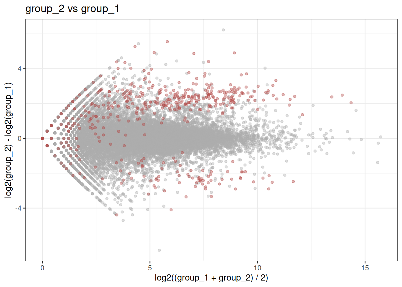
## 19548   452

The following MA plot highlights the simulated true DEGs.

Next, define a helper function that calculates the AUC from gene-level p-values. Smaller p-values are converted to larger ranking scores so that genes with stronger statistical evidence are ranked first.

library(pROC)

calc_auc <- function(is_deg, p_value) {
    p_value[is.na(p_value)] <- 1
    ranking_score <- -p_value
    roc_obj <- roc(is_deg, ranking_score)
    auc_value <- auc(roc_obj)
    as.numeric(auc_value)
}

5.3.1 Comparison with edgeR

This subsection uses simulated counts to compare a standard edgeR workflow with a DEGES-based normalization workflow followed by edgeR DEG testing.

First, run TMM normalization and a quasi-likelihood test with edgeR, then compute the AUC.

library(edgeR)

design <- model.matrix(~ group, data = x@exp_design)
d1 <- DGEList(counts = x@data, group = x@exp_design$group)
d1 <- calcNormFactors(d1)
d1 <- estimateDisp(d1, design)
fit1 <- glmQLFit(d1, design)
qlf1 <- glmQLFTest(fit1, coef = 2)
edger_output1 <- topTags(qlf1, n = nrow(d1$counts), sort.by = "none")$table

calc_auc(is_DEG, edger_output1$PValue)

## [1] 0.892813

Next, estimate normalization factors with the DEGES approach using calc_nf(). The result is converted to a edgeR object for the downstream DEG test, and AUC is computed from the resulting p-values.

x <- calc_nf(x, orm_func = norm_tmm, test_func = test_edger)

design <- model.matrix(~ group, data = x@exp_design)
d2 <- as_DGEList(x)
d2 <- estimateDisp(d2, design)
fit2 <- glmQLFit(d2, design)
qlf2 <- glmQLFTest(fit2, coef = 2)
edger_output2 <- topTags(qlf2, n = nrow(d2$counts), sort.by = "none")$table

calc_auc(is_DEG, edger_output2$PValue)

## [1] 0.8939575

5.3.2 Comparison with DESeq2

DESeq2 workflows can be evaluated in the same way. In normpatch, the built-in test_deseq2() function uses an LRT for DEG screening during DEGES-based normalization. Here, four workflows are compared:

RLE normalization, followed by a DESeq2 Wald test.
RLE normalization, followed by a DESeq2 LRT.
DEGES using RLE normalization and DESeq2 Wald screening, followed by a DESeq2 Wald test.
DEGES using RLE normalization and DESeq2 LRT screening, followed by a DESeq2 LRT.

First, run the DESeq2 Wald test and compute AUC.

library(DESeq2)

col_data <- x@exp_design
rownames(col_data) <- colnames(x@data)
design = ~ group

dds1 <- DESeqDataSetFromMatrix(countData = x@data, colData = col_data, design = design)
dds1 <- estimateSizeFactors(dds1)
dds1 <- estimateDispersions(dds1)
dds1 <- nbinomWaldTest(dds1)
deseq2_output_1 = as.data.frame(results(dds1))

calc_auc(is_DEG, deseq2_output_1$pvalue)

## [1] 0.8796549

Using the same input data, run DESeq2 with an LRT.

dds2 <- DESeqDataSetFromMatrix(countData = x@data, colData = col_data, design = design)
dds2 <- estimateSizeFactors(dds2)
dds2 <- estimateDispersions(dds2)
dds2 <- nbinomLRT(dds2, full = ~ group, reduced = ~ 1)
deseq2_output_2 = as.data.frame(results(dds2))

calc_auc(is_DEG, deseq2_output_2$pvalue)

## [1] 0.8799681

Next, evaluate a DEGES workflow that uses a Wald test during DEG screening. Because normpatch does not provide a built-in Wald screening function for calc_nf(), the example first defines test_deseq2_wald().

test_deseq2_wald <- function(x, exp_design, nf = NULL, ...) {
    if (is.null(nf)) nf <- rep(1, ncol(x))

    x <- as.matrix(x)
    exp_design <- as.data.frame(exp_design)
    rownames(exp_design) <- colnames(x)

    effective_lib_sizes <- nf * colSums(x)

    dds <- DESeqDataSetFromMatrix(
        countData = x,
        colData = exp_design,
        design = ~ group
    )
    sizeFactors(dds) <- effective_lib_sizes / mean(effective_lib_sizes)
    dds <- estimateDispersions(dds)
    dds <- nbinomWaldTest(dds)

    test_output <- as.data.frame(results(dds))
    p <- test_output$pvalue
    p[is.na(p)] <- 1
    q <- stats::p.adjust(p, method = "BH")

    data.frame(
        p_value = p,
        q_value = q,
        row.names = NULL,
        check.names = FALSE
    )
}


x3 <- calc_nf(x, norm_func = norm_rle, test_func = test_deseq2_wald)
dds3 <- as_DESeqDataSet(x3)
dds3 <- estimateDispersions(dds3)
dds3 <- nbinomWaldTest(dds3)
deseq2_output_3 = as.data.frame(results(dds3))

calc_auc(is_DEG, deseq2_output_3$pvalue)

## [1] 0.880846

Finally, evaluate the DEGES workflow that uses the DESeq2 LRT for DEG screening.

x4 <- calc_nf(x, norm_func = norm_rle, test_func = test_deseq2)
dds4 <- as_DESeqDataSet(x4)
dds4 <- estimateDispersions(dds4)
dds4 <- nbinomLRT(dds4, full = ~ group, reduced = ~ 1)
deseq2_output_4 = as.data.frame(results(dds4))

calc_auc(is_DEG, deseq2_output_4$pvalue)

## [1] 0.881102

The AUC values can then be summarized across the four workflows.

data.frame(
    pipeline = c("RLE + Wald", "RLE + LRT", "DEGES(Wald) + Wald", "DEGES(LRT) + LRT"),
    auc = c(
        calc_auc(is_DEG, deseq2_output_1$pvalue),
        calc_auc(is_DEG, deseq2_output_2$pvalue),
        calc_auc(is_DEG, deseq2_output_3$pvalue),
        calc_auc(is_DEG, deseq2_output_4$pvalue)
    )
)

##             pipeline       auc
## 1         RLE + Wald 0.8796549
## 2          RLE + LRT 0.8799681
## 3 DEGES(Wald) + Wald 0.8808460
## 4   DEGES(LRT) + LRT 0.8811020