4.2 Custom test functions

TbT (Kadota et al. 2012) is the original DEGES-based normalization workflow. It estimates normalization factors using TMM and screens candidate DEGs with baySeq. Because normpatch does not provide a built-in baySeq screening function, this section shows how to define a custom test function that reproduces the TbT workflow.

The test function should receive at least x as a count matrix, exp_design as a data frame of experimental design, and nf as normalization factors. It should return at least p-value (p_value) and q-value (q_value) columns in a data frame. Additional arguments can also be defined. For example, baySeq requires samplesize for bootstrapping during the test and cluster information through cl for parallel computation. The custom function adds these arguments and sets their default values.

library(baySeq)
library(parallel)

test_bayseq <- function(x, exp_design, nf, samplesize=10000, cl=NULL, ...) {
    d <- new("countData",
            data = x,
            replicates = exp_design$group,
            groups = list(NDE = rep(1, nrow(exp_design)), DE = exp_design$group),
            libsizes = nf * colSums(x))
    d@annotation <- data.frame(gene_id = 1:nrow(x))
    d <- getPriors.NB(d, estimation = "QL", samplesize = samplesize, cl = cl)
    d <- baySeq::getLikelihoods(d, pET = "BIC", cl = cl)
    test_stats <- topCounts(d, group = "DE", number = nrow(x))
    test_stats <- test_stats[order(test_stats$gene_id), ]
    p <- test_stats$FWER.DE
    q <- test_stats$FDR.DE
    p[is.na(p)] <- 1
    q[is.na(q)] <- 1
    data.frame(
        p_value = p,
        q_value = q,
        row.names = NULL, check.names = FALSE)
}

For the normalization step, the built-in norm_tmm() function can be used directly. After defining the test function, load the data and run normalization.

library(edgeR) # to use 'cpm' function
library(normpatch)

count_data <- read.table("data/ath.E-MTAB-4391.txt",
                         header = TRUE, sep = "\t", row.names = 1)
keep <- rowSums(cpm(count_data) > 5) > (ncol(count_data) / 2)
count_data <- as.matrix(count_data[keep, , drop = FALSE])

group <- sapply(strsplit(colnames(count_data), "_"), "[", 1)
exp_design <- data.frame(group = factor(group))

x <- newSeqCountData(count_data, exp_design = exp_design)

if(require("parallel")) {
    cl <- makeCluster(4)
} else {
    cl <- NULL
}

x <- calc_nf(x, norm_func = norm_tmm, test_func = test_bayseq,
             iter = 1, samplesize = 100, cl = cl)

if (!is.null(cl)) {
    stopCluster(cl)
}

Although test_bayseq() is primarily designed for use within calc_nf() during DEGES-based normalization, it also returns gene-level p-values and q-values. Therefore, it can also be used directly for DEG analysis.

if(require("parallel")) {
    cl <- makeCluster(4)
} else {
    cl <- NULL
}

test_stats <- test_bayseq(x@data, x@exp_design, x@meta$nf, samplesize = 100, cl = cl)

if (!is.null(cl)) {
    stopCluster(cl)
}

test_stats <- data.frame(gene_name = x@gene_names, test_stats)

head(test_stats)

##   gene_name   p_value     q_value
## 1 AT1G01010 1.0000000 0.636368002
## 2 AT1G01020 1.0000000 0.844859099
## 3 AT1G01040 1.0000000 0.840873144
## 4 AT1G01050 1.0000000 0.844212210
## 5 AT1G01060 1.0000000 0.238000519
## 6 AT1G01070 0.4016799 0.001076838

Next, visualize the test results by highlighting genes with q_value < 0.05 in the baySeq results.

is_deg <- test_stats$q_value < 0.05
gene_colors <- ifelse(is_deg, "#B24745", "#ADADAD")
plot_ma(x, col = gene_colors)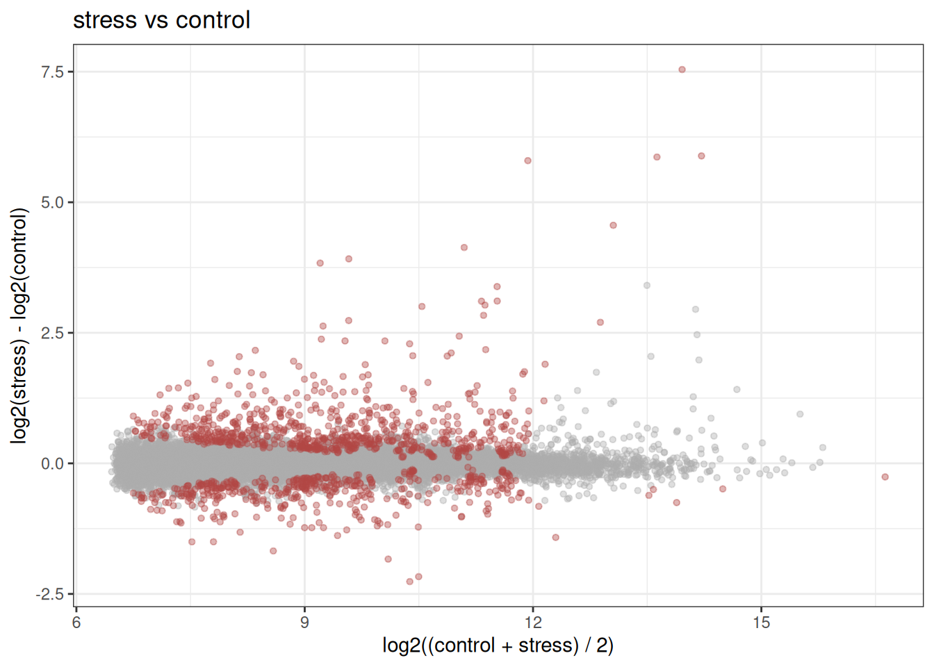

Here, samplesize = 100 is used only for the example. In practical analyses, use a larger value such as 10,000.