5.1 Generate simulated data

5.1.1 Standard usage

The simplest call to sim_gene_counts() creates a two-group count matrix containing 20,000 genes with three replicates per group. The function returns a SeqCountData object whose data slot contains the count matrix and whose exp_design slot contains the sample grouping.

library(normpatch)
set.seed(1)

x <- sim_gene_counts()
x

## SeqCountData object
##   genes:   10000
##   samples: 6
##   groups:  group_1, group_2
##   factors: not set

The simulation parameters are stored in x@meta$sim_params. They can be inspected through the slots of this object.

x@meta$sim_params@n_genes

## [1] 10000

x@meta$sim_params@p_DEG

## [1] 0.04 0.01

head(x@meta$sim_params@params)

##              mean         var dispersion distribution
## gene_1  0.1920639   0.2213313 0.79340066           NB
## gene_2  8.0588686  22.5053156 0.22244001           NB
## gene_3 71.7395714 202.3031325 0.02536906           NB
## gene_4  1.3072645  10.2536434 5.23504389           NB
## gene_5 19.8954781  49.8387062 0.07564668           NB
## gene_6  0.7843587   3.6913116 4.72507315           NB

head(x@meta$sim_params@fc)

##         group_1 group_2
## gene_1 1.892591       1
## gene_2 2.452496       1
## gene_3 3.613771       1
## gene_4 2.570786       1
## gene_5 2.812754       1
## gene_6 4.045095       1

Because the true mean and fold change parameters are known, DEG status can be defined directly from the simulated fold change matrix. The def_DEG() function marks genes as true DEGs when their largest between-group fold change is at least the cutoff specified by fc. fc defaults to 2 but can be changed.

is_DEG <- def_DEG(x)
head(is_DEG)

## gene_1 gene_2 gene_3 gene_4 gene_5 gene_6 
##  FALSE   TRUE   TRUE   TRUE   TRUE   TRUE

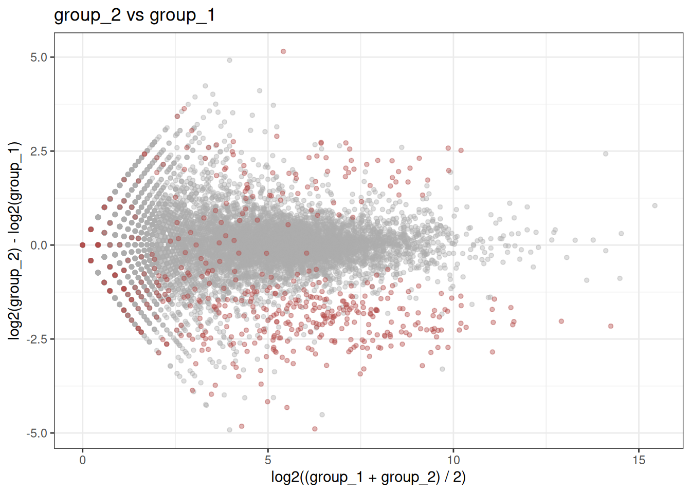
An MA plot provides a direct view of the simulated counts and the known true DEGs. Because plot_ma() uses normalized counts, estimate normalization factors before plotting. Here, simulated DEGs are highlighted in red and genes that are not DEGs are shown in gray.

x <- calc_nf(x)

gene_colors <- ifelse(is_DEG, "#B24745", "#ADADAD")
plot_ma(x, col = gene_colors)

The number of genes and the degree of DEG imbalance can be changed by specifying the corresponding arguments. In the following example, the second group contains a larger proportion of biased DEGs, and those genes are assigned a stronger fold change.

set.seed(1)

x <- sim_gene_counts(
    n_genes = 2000,
    n_replicates = c(4, 4),
    p_DEG = c(0.05, 0.15),
    fc_mean = c(8, 2),
    group_names = c("control", "stress")
)

is_DEG <- def_DEG(x, fc = 2)

x <- calc_nf(x)

gene_colors <- ifelse(is_DEG, "#B24745", "#ADADAD")
plot_ma(x, col = gene_colors)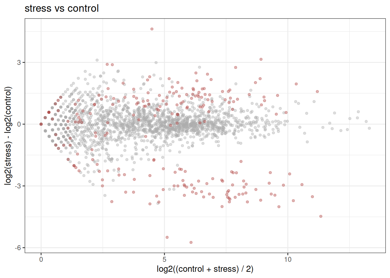

To generate a comparison with three groups, provide one replicate count, DEG proportion, and fold change value for each group. The example below creates three groups with different proportions of DEGs.

set.seed(1)

x <- sim_gene_counts(
    n_replicates = c(3, 3, 3),
    p_DEG = c(0.05, 0.10, 0.15),
    fc_mean = c(4, 4, 4),
    group_names = c("leaf", "root", "shoot")
)
x

## SeqCountData object
##   genes:   10000
##   samples: 9
##   groups:  leaf, root, shoot
##   factors: not set

5.1.2 Generate counts with randomized fold changes

5.1.2.1 Log-normal fold changes

By default, sim_gene_counts() samples fold changes for genes assigned as DEGs from a lognormal distribution. This makes the simulated effect sizes heterogeneous, which is closer to typical RNA-seq datasets than assigning the same fold change to every DEG.

With randomized fold changes, fc_mean is interpreted as the mean fold change for genes assigned as DEGs. For this distribution, the fc_sd argument controls the spread of the sampled values as the standard deviation on the natural log fold change scale.

set.seed(1)

x <- sim_gene_counts(
    fc_dist = "lognormal",
    fc_mean = c(4, 4),
    fc_sd = 0.5,
    group_names = c("control", "stress")
)

true_fc <- x@meta$sim_params@fc[, "stress"]
summary(true_fc[true_fc != 1])

##    Min. 1st Qu.  Median    Mean 3rd Qu.    Max. 
##   1.179   2.378   3.563   3.860   4.834  11.244

The sampled fold-change matrix is stored in x@meta$sim_params@fc. The def_DEG() function uses these fold changes to define the true DEG status. Because this classification is based on a fold-change cutoff, the resulting number of true DEGs may differ from the proportion specified by the p_DEG argument.

is_DEG <- def_DEG(x, fc = 2)
table(is_DEG)

## is_DEG
## FALSE  TRUE 
##  9554   446

x <- calc_nf(x, iter = 0)

gene_colors <- ifelse(is_DEG, "#B24745", "#ADADAD")
plot_ma(x, col = gene_colors) + ggtitle("lognormal")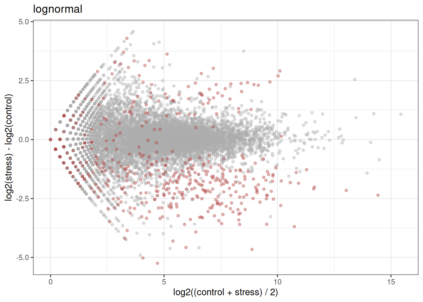

5.1.2.2 Gamma fold changes

The gamma option provides another positive distribution for fold changes. Here, the mean fold change is again set by fc_mean, while fc_sd controls the coefficient of variation.

set.seed(1)

x <- sim_gene_counts(
    fc_dist = "gamma",
    fc_mean = c(4, 4),
    fc_sd = 0.5,
    group_names = c("control", "stress")
)

true_fc <- x@meta$sim_params@fc[, "stress"]
summary(true_fc[true_fc != 1])

##    Min. 1st Qu.  Median    Mean 3rd Qu.    Max. 
##   1.005   2.570   3.851   4.108   5.259  11.532

x <- calc_nf(x, iter = 0)

is_DEG <- def_DEG(x, fc = 2)
gene_colors <- ifelse(is_DEG, "#B24745", "#ADADAD")
plot_ma(x, col = gene_colors) + ggtitle("gamma")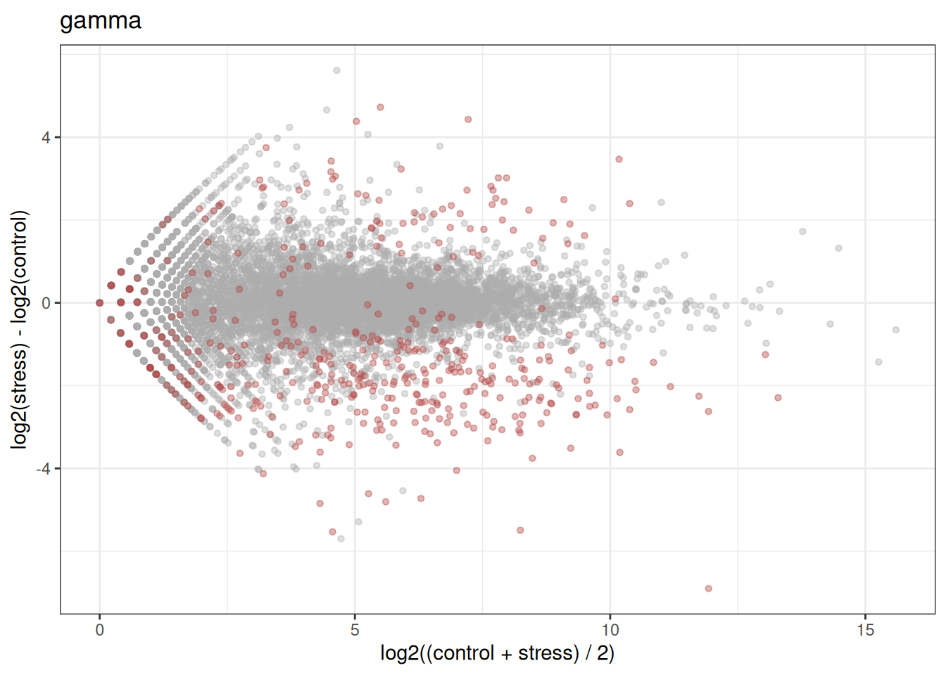

5.1.2.3 Fixed fold changes

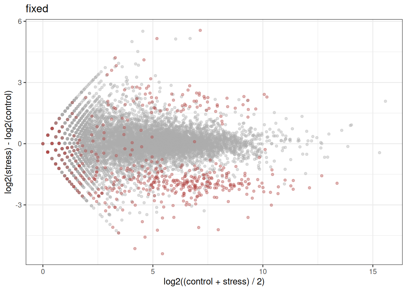
Fixed fold changes are still available for controlled simulations. Set fc_dist = "fixed" when every DEG assigned to a group should receive the exact value in fc_mean.

set.seed(1)

x <- sim_gene_counts(
    fc_dist = "fixed",
    fc_mean = c(4, 4),
    group_names = c("control", "stress")
)

true_fc <- x@meta$sim_params@fc[, "stress"]
unique(true_fc[true_fc != 1])

## [1] 4

x <- calc_nf(x, iter = 0)

is_DEG <- def_DEG(x, fc = 2)
gene_colors <- ifelse(is_DEG, "#B24745", "#ADADAD")
plot_ma(x, col = gene_colors) + ggtitle("fixed")