3.1 Two-group comparison
A two-group comparison is one of the most common RNA-seq experimental designs. Examples include treatment versus control, mutant versus wild type, and one tissue versus another tissue. This section explains how to perform a two-group comparison by using normpatch and edgeR or DESeq2. The example used here can be downloaded from Expression Atlas with the accession number E-MTAB-4391, which profiles Arabidopsis thaliana roots grown under iron-deficient and control conditions (Li and Lan 2015).
atlas <- getAtlasData("E-MTAB-4391")
se <- atlas[[1]]$rnaseq

count_data <- as.matrix(assay(se, "counts"))
head(count_data)
## SRR1524935 SRR1524938 SRR1524940 SRR1524941 SRR1524945 SRR1524946
## AT1G01010 558 457 392 570 621 593
## AT1G01020 442 345 274 403 435 436
## AT1G01030 33 27 21 24 37 34
## AT1G01040 1149 843 703 1058 1038 1047
## AT1G01046 12 12 19 17 16 17
## AT1G01050 2013 1744 1585 1816 1983 2122## [1] "AT1G01010" "AT1G01020" "AT1G01030" "AT1G01040" "AT1G01046" "AT1G01050"## AtlasAssayGroup organism ecotype organism_part developmental_stage age environmental_stress
## SRR1524935 g1 Arabidopsis thaliana Col-0 root seedling 13 day control
## SRR1524938 g1 Arabidopsis thaliana Col-0 root seedling 13 day control
## SRR1524940 g1 Arabidopsis thaliana Col-0 root seedling 13 day control
## SRR1524941 g2 Arabidopsis thaliana Col-0 root seedling 13 day limited iron regimen
## SRR1524945 g2 Arabidopsis thaliana Col-0 root seedling 13 day limited iron regimen
## SRR1524946 g2 Arabidopsis thaliana Col-0 root seedling 13 day limited iron regimenGenes with little or no expression provide limited statistical information and can reduce power in DEG analysis. Here, we retain genes with more than 5 CPM in more than half of the samples for the downstream analysis.
keep <- rowSums(cpm(count_data) > 5) > ncol(count_data) / 2
count_data <- count_data[keep, , drop = FALSE]
count_data <- as.matrix(count_data)
dim(count_data)
## [1] 15691 6Next, prepare the sample information.
The experimental condition is stored in a data frame named exp_design.
Each row of exp_design represents one sample and must match the columns of count_data in the same order.
##                  group
## 1              control
## 2              control
## 3              control
## 4 limited iron regimen
## 5 limited iron regimen
## 6 limited iron regimen
The count matrix and sample information are then combined into a SeqCountData object.
The calc_nf() function estimates normalization factors using DEGES,
which repeatedly performs four steps:
- Estimate provisional normalization factors.
- Identify candidate DEGs.
- Exclude those candidate genes.
- Recalculate the normalization factors.
By default, calc_nf() uses TMM normalization and a edgeR
quasi-likelihood test during DEG elimination.
The computed normalization factors can be accessed through the meta slot.
They are used together with the library sizes when fitting the downstream statistical model.
## SRR1524935 SRR1524938 SRR1524940 SRR1524941 SRR1524945 SRR1524946
##  1.0171957  1.0119893  1.0127063  0.9754117  0.9758077  1.0068892
To identify DEGs with these normalization factors,
use as_DGEList() to convert the current object to a edgeR DGEList,
then fit the statistical model with edgeR.
d <- as_DGEList(x)

design = model.matrix(~ group, data = exp_design)

d <- estimateDisp(d, design = design)
fit <- glmQLFit(d, design = design)
qlf <- glmQLFTest(fit, coef = 2)
After the test, extract the results for all genes.
##                 logFC   logCPM           F       PValue         FDR
## AT1G01010  0.11660865 4.900775  2.93104328 0.1172343516 0.307612744
## AT1G01020  0.04573917 4.450448  0.37448439 0.5540350724 0.744167464
## AT1G01040  0.00838787 5.767843  0.01806385 0.8957136213 0.952176428
## AT1G01050 -0.08956274 6.727516  1.49765070 0.2486922575 0.474723870
## AT1G01060  0.14418796 5.814221  5.95276916 0.0345363122 0.146819094
## AT1G01070 -0.42450045 4.969825 29.84581942 0.0002619819 0.005735274
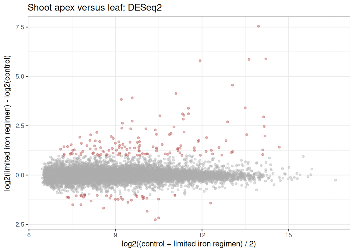
An MA plot displays the log fold change of each gene against its average expression level. The following example highlights genes with a false discovery rate (FDR) below 0.01 and an absolute log2 fold change greater than 1.
is_deg <- (test_stats$FDR < 0.01) & (abs(test_stats$logFC) > 1)
gene_colors <- ifelse(is_deg, "#B24745", "#ADADAD")
plot_ma(x, col = gene_colors)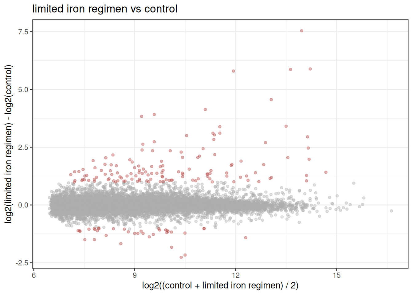
The significance thresholds used here are examples. Appropriate thresholds depend on the study design and should be selected before interpreting the results.
The same two-group workflow can be run with DESeq2.
In this case, estimate DEGES normalization factors using the RLE
normalization method and DESeq2-based DEG elimination by setting
norm_func and test_func to functions compatible with DESeq2.
x <- newSeqCountData(count_data, exp_design = exp_design)
x <- calc_nf(x, norm_func = norm_rle, test_func = test_deseq2)

dds <- as_DESeqDataSet(x)

dds <- DESeq2::estimateDispersions(dds)
dds <- DESeq2::nbinomLRT(dds, full = ~ group, reduced = ~ 1)
test_stats <- DESeq2::results(dds)
head(test_stats)
## log2 fold change (MLE): group limited.iron.regimen vs control
## LRT p-value: '~ group' vs '~ 1'
## DataFrame with 6 rows and 6 columns
## baseMean log2FoldChange lfcSE stat pvalue padj
## <numeric> <numeric> <numeric> <numeric> <numeric> <numeric>
## AT1G01010 531.300 0.11472219 0.0992470 1.33581569 2.47773e-01 0.558612260
## AT1G01020 388.012 0.04414463 0.1099909 0.16189054 6.87422e-01 0.881711568
## AT1G01040 970.648 0.00638054 0.0854434 0.00593062 9.38615e-01 0.979644619
## AT1G01050 1892.052 -0.09145441 0.0849572 1.15900423 2.81672e-01 0.596694711
## AT1G01060 1002.555 0.14258307 0.0831626 2.93822248 8.65059e-02 0.316571522
## AT1G01070 560.087 -0.42687441 0.1021470 17.44645540 2.95515e-05 0.000600638With this design, full = ~ group and reduced = ~ 1,
the LRT compares the full model containing group with the reduced model that does not contain group.
It therefore tests whether group membership explains a significant amount of gene expression variation.
The results can also be visualized with an MA plot.
is_deg <- (test_stats$padj < 0.05) & (abs(test_stats$log2FoldChange) > 1)
gene_colors <- ifelse(is_deg, "#B24745", "#ADADAD")

ma_plot <- plot_ma(x, col = gene_colors)
ma_plot + ggtitle("Shoot apex versus leaf: DESeq2")