5.1 Simulating Allotetraploid Data
The hespresso package provides functions to simulate artificial read counts for allotetraploid and allohexaploid species. By default, the simulation generates read counts for an allotetraploid with 10,000 homeologs across two conditions, each with three biological replicates. The mean and dispersion parameters are estimated from real RNA-seq data from an allotetraploid Cardamine flexuosa dataset (Akiyama et al. 2021).
To generate a simulated dataset with default options, run as follows.
## # 2 subgenome sets (A, B)
## # 10000 homeolog tuples
## ---------------------
## Experiment Design:
##     group replicate
## 1 group_1         1
## 2 group_1         2
## 3 group_1         3
## 4 group_2         1
## 5 group_2         2
## 6 group_2         3
## ---------------------
## > subgenome: A
##        group_1__1 group_1__2 group_1__3 group_2__1 group_2__2 group_2__3
## gene_1         27         22         16         14         14         22
## gene_2        278          4         12         87        113         93
## gene_3        614        316        433        437        228        631
## gene_4        360        341        311        359        237        411
## gene_5        138         42        214        150        189        165
## gene_6       1028       1063       1171        383        385        342
## +++++++++++++++++++++
## > subgenome: B
##        group_1__1 group_1__2 group_1__3 group_2__1 group_2__2 group_2__3
## gene_1          9         21         11         21         19         21
## gene_2        124        107        123        218        187        200
## gene_3        162        149        206        180        235        259
## gene_4        373        329        384        353        269        374
## gene_5         63         45         69         75         49         43
## gene_6        101         93        102         67         98         83
## ---------------------
Options can be flexibly customized by users. For example, to simulate data with 1,000 homeologs and 5 replicates per condition, run as follows.
## # 2 subgenome sets (A, B)
## # 1000 homeolog tuples
## ---------------------
## Experiment Design:
##      group replicate
## 1  group_1         1
## 2  group_1         2
## 3  group_1         3
## 4  group_1         4
## 5  group_1         5
## 6  group_2         1
## 7  group_2         2
## 8  group_2         3
## 9  group_2         4
## 10 group_2         5
## ---------------------
## > subgenome: A
##        group_1__1 group_1__2 group_1__3 group_1__4 group_1__5 group_2__1 group_2__2 group_2__3 group_2__4 group_2__5
## gene_1         59         58         58         51         47         70         43         71         53         45
## gene_2          8          2          5         36         13          6          9          6          7          6
## gene_3          4          4          4          4          9          0          0          1          8          0
## gene_4         27         34         34         28         18          8          6         10         18         15
## gene_5         52         43         32         54         37         31         10          5         22         10
## gene_6       1273       1749       1696       2733       1867       1506       1748       1757       2009       1948
## +++++++++++++++++++++
## > subgenome: B
##        group_1__1 group_1__2 group_1__3 group_1__4 group_1__5 group_2__1 group_2__2 group_2__3 group_2__4 group_2__5
## gene_1         12          3         36          0          7         23         21         19         26         13
## gene_2          6          3          5          2          7          0          0          0          0          0
## gene_3          6          7          9         10          4          8          8         12          8          8
## gene_4         33         12          2          0          1          7          5         11          2          8
## gene_5        202        136        178        156        189        188        167        163        167        153
## gene_6        793        842        918        800        937        989       1112        845        945        992
## ---------------------
Parameters used for simulating read counts are stored in the x object
returned by the sim_homeolog_counts() function.
Users can access these parameters via the @meta slot of the x object.
For example, x@meta contains the following information:
## [1] "n_subgenomes" "n_genes" "n_groups" "n_replicates" "params_population" "params" "nls" "mu" "her"To retrieve the ground-truth means used for the simulation,
users can access the mu slot as follows.
## [1] "group_1" "group_2"## A B
## gene_1 56.491374 17.328355
## gene_2 8.006597 4.818938
## gene_3 5.944184 6.766986
## gene_4 28.174125 7.362780
## gene_5 44.853340 166.388422
## gene_6 1902.944015 899.045310## A B
## gene_1 47.044944 17.335548
## gene_2 7.043161 3.587883
## gene_3 4.899969 6.314536
## gene_4 12.831738 7.463493
## gene_5 19.546177 159.654936
## gene_6 1907.297324 958.044278The dispersion parameters used in the simulation are estimated from
the relationship between mean and dispersion in a real RNA-seq dataset.
The fitted model function can be accessed via the nls slot.
## $nls
## Nonlinear regression model
##   model: y ~ a * x * x + b * x + c
##    data: data.frame(x = log10(p_pop$mean), y = log10(p_pop$variance))
##      a      b      c
## 0.2551 0.5329 0.4820
##  residual sum-of-squares: 63935
##
## Number of iterations to convergence: 1
## Achieved convergence tolerance: 6.097e-09
##
## $nls_variance
## [1] 0.4873068
Additionally, the ground-truth homeolog expression ratios can be calculated manually
from the ground-truth means, or they can be retrieved directly from the her slot, as follows.
## [1] "group_1" "group_2"## A B
## gene_1 0.7652612 0.2347388
## gene_2 0.6242700 0.3757300
## gene_3 0.4676347 0.5323653
## gene_4 0.7928131 0.2071869
## gene_5 0.2123318 0.7876682
## gene_6 0.6791404 0.3208596## A B
## gene_1 0.7307329 0.2692671
## gene_2 0.6625089 0.3374911
## gene_3 0.4369314 0.5630686
## gene_4 0.6322539 0.3677461
## gene_5 0.1090740 0.8909260
## gene_6 0.6656440 0.3343560Using this information,
users can define homeologs that show significant changes in expression ratios between conditions.
Alternatively, the def_sigShift() function can automatically identify homeologs
with significant shifts without the need for manual calculations.
For example, to identify homeologs with a maximum absolute ratio difference (Dmax) greater than 0.2
or a maximum odds ratio (ORmax) exceeding 2.0, use the following code.
x <- sim_homeolog_counts()

is_sig <- def_sigShift(x, Dmax = 0.2, ORmax = 2, operator = "OR")
table(is_sig)
## is_sig
## FALSE TRUE
## 9260 740The output shows the number of homeologs meeting these thresholds.
To visualize the distribution of expression ratios across conditions,
use the plot_HER_distr() function.
This returns a list of histograms, one per condition,
with ratios calculated by default for the first subgenome (base = 1).
Since the simulated dataset contains two groups,
the plot_HER_distr() function returns two histograms.
## [1] "group_1" "group_2"To display the distributions for each group, run as follows.
library(ggplot2)
library(gridExtra)

grid.arrange(distr_plots[["group_1"]] + ggtitle("group_1"),
             distr_plots[["group_2"]] + ggtitle("group_2"),
             ncol = 2)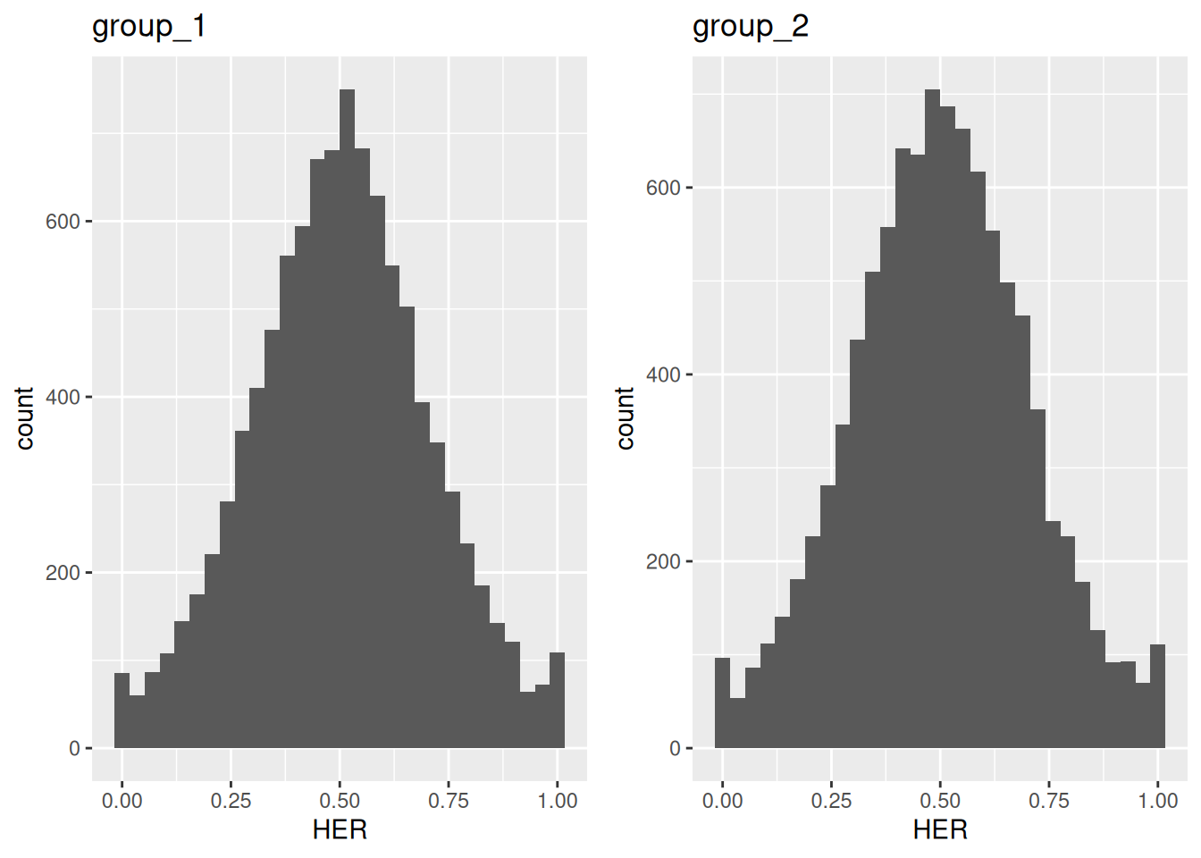
Figure 5.1: Distribution of homeolog expression ratios in two simulated groups.
To compare expression ratios between groups, use the plot_HER() function,
which by default plots ratios for the first subgenome in a scatter plot.
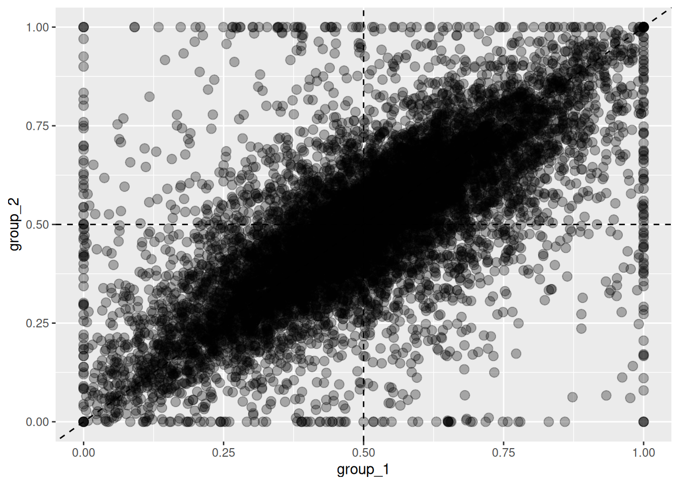
Figure 5.2: Changes in homeolog expression ratios between two groups. Each point represents the expression ratio in group 1 (x-axis) and group 2 (y-axis).
If the dataset was generated using sim_homeolog_counts(),
ground-truth significant shifts can be highlighted as follows using the def_sigShift() function.
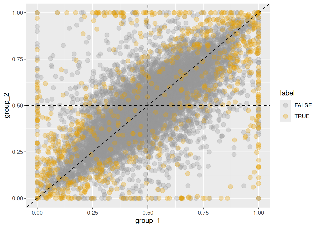
Figure 5.3: Changes in homeolog expression ratios between two groups. Orange points indicate homeologs with significant changes in expression ratios, while gray points represent those without significant changes.