3.2 Allohexaploid T. aestivum
3.2.1 Introduction
Bread wheat, Triticum aestivum (2n = 6x = 42, AABBDD), is one of the world’s most important crops and also serves as a model for studying allopolyploid species. It originated through hybridization among three diploid progenitor species, Triticum urartu (2n = 2x = 14, AA), an unknown species related to Aegilops speltoides (2n = 2x = 14; SS, which is thought to be the progenitor of BB), and Aegilops tauschii (2n = 2x = 14, DD), containing three distinct subgenomes (IWGSC 2018; Levy and Feldman 2022; Zhao et al. 2023). To demonstrate the applicability of HOBIT to allohexaploid species, we present a case study using wheat RNA-seq data to detect homeologs with shifts in expression ratios between two tissues, shoot apex and leaf (Yang et al. 2021).
3.2.2 Data Preparation
In this example, 500 homeolog triads were randomly selected from the original dataset.
The expression data can be loaded from the following file (t_aestivum.w20.mini.txt.gz).
Users may also choose to load the full dataset, which is stored
in the data directory, for analysis.
gexp <- read.table("../data/t_aestivum.w20.mini.txt.gz",
                   header = TRUE, sep = "\t", row.names = 1)
head(gexp)
## shootapex_1 shootapex_2 shootapex_3 leaf_1 leaf_2 leaf_3
## TraesCS1A02G024700 65 69 53 63 51 39
## TraesCS1A02G029300 206 164 227 1439 1125 1444
## TraesCS1A02G046900 49 44 41 1 0 0
## TraesCS1A02G063600 111 70 77 4 10 6
## TraesCS1A02G067300 1212 1247 1274 22 21 24
## TraesCS1A02G072800 133 143 143 0 0 0Next, load the mapping table that links each gene to its corresponding homeolog triads. Since wheat has three subgenomes (i.e., A, B, and D), the table contains three columns, with each column representing one subgenome.
mapping_table <- read.table("../data/t_aestivum.homeolog.txt.gz",
                            header = TRUE, sep = "\t")
head(mapping_table)
## A B D
## 1 TraesCS1A02G000800 TraesCS6B02G173200LC TraesCS5D02G023700
## 2 TraesCS1A02G000900 TraesCS6B02G117800 TraesCS7D02G119300
## 3 TraesCS1A02G001600 TraesCS1B02G320300 TraesCS7D02G148100LC
## 4 TraesCS1A02G001900 TraesCS1B02G000800 TraesCS1D02G003900
## 5 TraesCS1A02G002000 TraesCS1B02G000900 TraesCS1D02G004000
## 6 TraesCS1A02G002100 TraesCS1B02G001000 TraesCS1D02G004100We then construct an ExpMX class object using the newExpMX() function.
This converts the gene expression matrix (gexp)
into a homeolog expression matrix based on the mapping table (mapping_table).
## # 3 subgenome sets (A, B, D)
## # 500 homeolog tuples
## ---------------------
## Experiment Design:
##   group
## 1  apex
## 2  apex
## 3  apex
## 4  leaf
## 5  leaf
## 6  leaf
## ---------------------
## > subgenome: A
##      [,1] [,2] [,3] [,4] [,5] [,6]
## [1,]   65   69   53   63   51   39
## [2,]  206  164  227 1439 1125 1444
## [3,]   49   44   41    1    0    0
## [4,]  111   70   77    4   10    6
## [5,] 1212 1247 1274   22   21   24
## [6,]  133  143  143    0    0    0
## +++++++++++++++++++++
## > subgenome: B
##      [,1] [,2] [,3] [,4] [,5] [,6]
## [1,]   91   92  119   60   87   64
## [2,]    4    0    0  622  285  383
## [3,]   85  118  100    0    1    7
## [4,]  122  108  116    5   16   12
## [5,] 1540 1426 1530   18   21   35
## [6,]  158  168  163    0    0    0
## +++++++++++++++++++++
## > subgenome: D
##      [,1] [,2] [,3] [,4] [,5] [,6]
## [1,]   89  107   83  180  150  111
## [2,]  155  232  176 2639 1860 2286
## [3,]  107  115   82    0    0    0
## [4,]   59   48   63    4    6    4
## [5,] 1163 1097 1127   18   10   27
## [6,]  137  139  124    1    1    0
## ---------------------
Before performing the test,
we normalize the raw read counts using the TMM method (Robinson and Oshlack 2010)
to adjust for differences in library size.
However, if the expression data (gexp) has already been normalized (e.g. FPKM),
this step can be skipped.
To visualize the distributions of homeolog expression ratios, use the plot_HER_distr() function.
By default, the expression ratio is calculated as the proportion contributed
by the first subgenome relative to all subgenomes.
In this dataset, the first subgenome corresponds to the A-subgenome,
as indicated by the first column of the mapping table (mapping_table).
## [1] "apex" "leaf"library(ggplot2)
library(gridExtra)
grid.arrange(distr_plots_A[["apex"]] + ggtitle("A-ratio in apex sample"),
distr_plots_A[["leaf"]] + ggtitle("A-ratio in leaf sample"),
ncol = 2)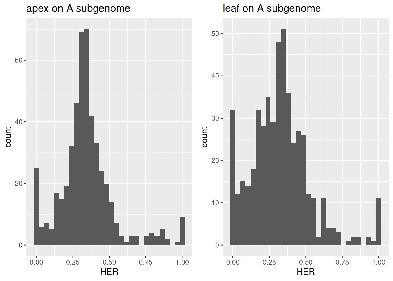
Figure 3.6: Distribution of homeolog expression ratios between shoot apex and leaf in the A-subgenome of wheat.
To calculate the ratios for the second and third subgenomes
(i.e., B-subgenome and D-subgenome), set base = 2 and base = 3, respectively.
distr_plots_B <- plot_HER_distr(x, base = 2)
distr_plots_D <- plot_HER_distr(x, base = 3)

grid.arrange(distr_plots_A[["apex"]] + ggtitle("A-ratio in apex sample"),
             distr_plots_A[["leaf"]] + ggtitle("A-ratio in leaf sample"),
             distr_plots_B[["apex"]] + ggtitle("B-ratio in apex sample"),
             distr_plots_B[["leaf"]] + ggtitle("B-ratio in leaf sample"),
             distr_plots_D[["apex"]] + ggtitle("D-ratio in apex sample"),
             distr_plots_D[["leaf"]] + ggtitle("D-ratio in leaf sample"),
             ncol = 2)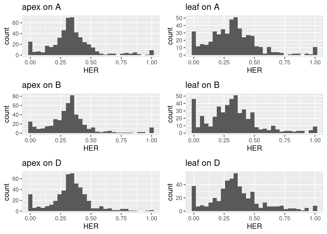
Figure 3.7: Distribution of homeolog expression ratios between shoot apex and leaf across all subgenomes.
Histogram peaks at one-third for all subgenomes indicate that most homeologs in wheat are equally expressed from the three subgenomes.
3.2.3 Statistical Test
After visually inspecting the distributions of homeolog expression ratios,
use the hobit() function to identify homeologs
showing significant changes in expression ratios between shoot apex and leaf tissues.
This step takes approximately five minutes using eight threads and may vary depending on hardware performance.
##                 gene       pvalue       qvalue   raw_pvalue   raw_qvalue D__A__(apex-leaf) D__B__(apex-leaf) D__D__(apex-leaf) OR__A__(apex/leaf) OR__B__(apex/leaf) OR__D__(apex/leaf)       Dmax     ORmax theta0__A  theta0__B theta0__D theta1__A__apex theta1__B__apex theta1__D__apex theta1__A__leaf theta1__B__leaf theta1__D__leaf  logLik_H0  logLik_H1
## 1 TraesCS1A02G024700 2.593448e-02 6.206210e-02 5.402719e-03 1.292889e-02        0.05225261        0.12931477       -0.17957945          1.3618972         1.81473169          0.4800414 0.17957945  2.083154 0.2176949 0.32799422 0.4522615       0.2426203     0.392523300       0.3624750       0.1911632       0.2626183      0.54229056  -82.00955  -76.91713
## 2 TraesCS1A02G029300 5.087286e-13 1.287887e-11 2.668237e-18 6.754852e-17        0.17633649       -0.10552727       -0.06850617          2.0819265         0.03039051          0.7587723 0.17633649 32.905009 0.4211210 0.05706343 0.5204076       0.5107931     0.003800232       0.4850465       0.3317129       0.1098155      0.55397535 -140.90456 -100.61030
## 3 TraesCS1A02G046900 1.823111e-08 2.740363e-07 8.643887e-12 1.299284e-10        0.03326121       -0.35286349        0.34666298          1.2803668         0.21437911         11.0184941 0.35286349 11.018494 0.1639428 0.58625867 0.2369349       0.1805322     0.408985260       0.4091255       0.1456108       0.7641598      0.05922983  -70.68208  -45.32985
## 4 TraesCS1A02G063600 6.040507e-01 7.430906e-01 4.864531e-01 5.984244e-01        0.03687783       -0.03443163        0.01102251          1.1873219         0.87013947          1.0682012 0.03687783  1.187322 0.3143956 0.46406366 0.2152589       0.3317806     0.445649955       0.2206155       0.2963886       0.4803274      0.20920804  -59.75544  -59.03119
## 5 TraesCS1A02G067300 7.622636e-02 1.449205e-01 2.523207e-02 4.797086e-02       -0.00731712        0.01507253        0.00400522          0.9672774         1.06633029          1.0197250 0.01507253  1.066330 0.3256640 0.37848541 0.2897259       0.3217743     0.386167995       0.2916401       0.3295151       0.3703209      0.28722329  -88.04429  -84.43668
## 6 TraesCS1A02G072800 7.353369e-10 1.473738e-08 8.781360e-14 1.759931e-12        0.15873297        0.21249363       -0.29717100          2.4517067         3.08731747          0.2888406 0.29717100  3.462118 0.2428002 0.26800078 0.4538831       0.3206853     0.373556005       0.3045184       0.1614315       0.1620491      0.60418619  -71.38397  -41.20234
Note that the pvalue and qvalue columns in x_output may contain NA values.
This happens when at least one gene in a homeolog triad is not expressed in one or more conditions,
making it impossible to calculate expression ratios.
As a result, the statistical test cannot be performed for those triads.
These NA values may affect sorting or counting the number of significant homeolog triads.
Therefore, we recommend replacing NA with 1 (i.e., non-significant)
before performing downstream analyses.
The output can be sorted in ascending order of p-values using the following code.
##                   gene       pvalue       qvalue   raw_pvalue   raw_qvalue D__A__(apex-leaf) D__B__(apex-leaf) D__D__(apex-leaf) OR__A__(apex/leaf) OR__B__(apex/leaf) OR__D__(apex/leaf)      Dmax     ORmax theta0__A theta0__B theta0__D theta1__A__apex theta1__B__apex theta1__D__apex theta1__A__leaf theta1__B__leaf theta1__D__leaf logLik_H0  logLik_H1
## 441 TraesCS7A02G209600 1.930125e-36 9.283901e-34 8.824101e-52 4.244392e-49        0.47038827        -0.7237735         0.2526528        44.52068399         0.01348721         18.3706073 0.7237735 74.144346 0.2579986 0.5939245 0.1473389       0.4929791      0.23123061       0.2737861      0.02146361       0.9572127      0.02014443 -186.7511  -69.36264
## 62  TraesCS1A02G445500 8.145322e-24 1.958950e-21 9.857762e-34 2.370792e-31       -0.02356230         0.2709820        -0.2382380         0.88414204         4.41087883          0.3760738 0.2709820  4.410879 0.2601458 0.2700551 0.4654294       0.2478861      0.40555679       0.3463748      0.27160212       0.1344130      0.58437523 -175.2964  -99.49567
## 299 TraesCS5A02G022200 1.096225e-22 1.757614e-20 4.052131e-32 6.496917e-30        0.35939003        -0.1503651        -0.2057783         5.36695600         0.18884623          0.4323623 0.3593900  5.366956 0.3599959 0.1195890 0.5195800       0.5400245      0.04354448       0.4157628      0.17861479       0.1948074      0.62286237 -182.3615 -110.15788
## 268 TraesCS4A02G250600 7.105293e-19 8.544115e-17 1.139493e-26 1.370240e-24       -0.05161338         0.2759468        -0.1707044         0.77480739         4.48096777          0.4898167 0.2759468  4.480968 0.2848769 0.2724789 0.4138247       0.2600280      0.40976656       0.3298487      0.31018767       0.1346049      0.49911507 -112.2118  -52.27832
## 422 TraesCS6A02G314400 3.241271e-18 3.118103e-16 9.972097e-26 9.593158e-24       -0.30870543         0.2161396         0.1047919         0.27887534         3.29952612          1.8040179 0.3087054  3.585832 0.4982453 0.2563342 0.2379452       0.3440264      0.36470117       0.2901437      0.65287900       0.1479618      0.18425254 -143.4203  -85.90735
## 36  TraesCS1A02G247200 5.431856e-18 4.354538e-16 2.086080e-25 1.672341e-23       -0.46493242         0.2994201         0.1650345         0.03911654        33.37836055         11.0734370 0.4649324 33.378361 0.7259690 0.1665420 0.1060697       0.4941075      0.31622874       0.1883364      0.96144335       0.0137202      0.02070764 -110.0735  -53.49287
Next, we visualize changes in expression ratios of the first subgenome between the two tissues. In the plot, homeologs with q-values less than 0.01 are highlighted.
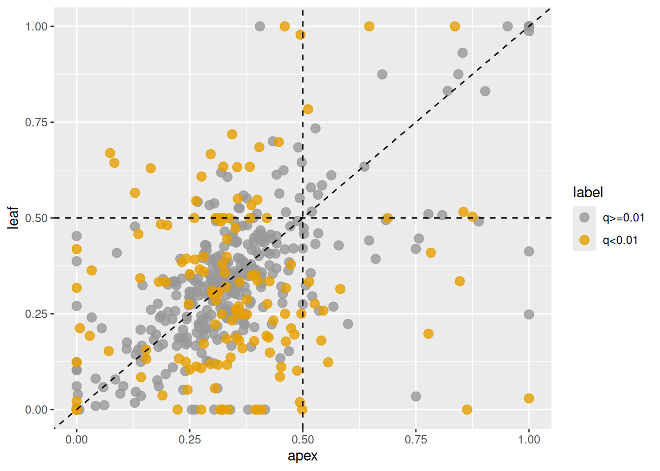
Figure 3.8: Changes in homeolog expression ratios of the A-subgenome between shoot apex and leaf tissues. Each point represents the ratio in shoot apex (x-axis) and leaf (y-axis). Orange points indicate homeologs with significant changes, gray points indicate homeologs without significant changes.
To change the subgenome used for calculating expression ratios,
set the base argument to the corresponding subgenome number.
For example, to use the second subgenome, run the following.
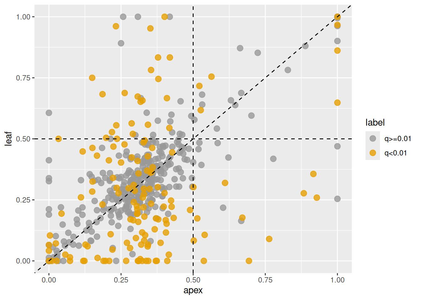
Figure 3.9: Changes in homeolog expression ratios of the B-subgenome between shoot apex and leaf tissues. Each point represents the ratio in shoot apex (x-axis) and leaf (y-axis). Orange points indicate homeologs with significant changes, gray points indicate homeologs without significant changes.
Note that expression ratios in the plots are calculated for the selected subgenome, while highlighted homeologs are those that meet the significance threshold in any subgenome. As a result, some homeologs may appear highlighted even if they show only minor changes in the plots, because they may have significantly altered expression ratios in another subgenome.
3.2.4 Combining Subgenomes
Users who want to test expression ratios
between the combined A- and B-subgenomes versus the D-subgenome
can first merge the expression of the A and B homeologs
using the combine_hexp() function.
After the merging step, statistical tests can be performed on the resulting dataset.
Assuming the A- and B-subgenomes are stored as the first and second subgenomes
in the x object (as defined in the mapping_table),
set subgenomes = c(1, 2) to combine them.
## # 2 subgenome sets (D, A+B)
## # 500 homeolog tuples
## ---------------------
## Experiment Design:
##   group
## 1  apex
## 2  apex
## 3  apex
## 4  leaf
## 5  leaf
## 6  leaf
## ---------------------
## > subgenome: D
##           [,1]      [,2]      [,3]        [,4]        [,5]        [,6]
## [1,]  69.91587  92.91579  69.32209  233.369104  182.885467  141.103672
## [2,] 121.76359 201.46227 146.99623 3421.450364 2267.779789 2905.972925
## [3,]  84.05615  99.86276  68.48688    0.000000    0.000000    0.000000
## [4,]  46.34872  41.68185  52.61797    5.185980    7.315419    5.084817
## [5,] 913.61969 952.60392 941.27700   23.336910   12.192364   34.322515
## [6,] 107.62330 120.70369 103.56553    1.296495    1.219236    0.000000
## +++++++++++++++++++++
## > subgenome: A+B
##           [,1]      [,2]      [,3]        [,4]        [,5]       [,6]
## [1,]  122.5492  139.8079  143.6554  159.468888  168.254630  130.93404
## [2,]  164.9700  142.4130  189.5917 2672.076241 1719.123389 2322.49017
## [3,]  105.2666  140.6762  117.7640    1.296495    1.219236    8.89843
## [4,]  183.0382  154.5702  161.1947   11.668455   31.700148   22.88168
## [5,] 2161.8929 2321.1579 2341.9172   51.859801   51.207931   75.00105
## [6,]  228.6013  270.0636  255.5730    0.000000    0.000000    0.00000
## ---------------------
In this case, the combined A- and B-subgenomes are appended as the last subgenome,
so the subgenome order in x_ABvsD becomes D and A+B.
The distribution of homeolog expression ratios can
then be visualized using the plot_HER_distr() function.
By default, the ratios are calculated for the D-subgenome,
as D-subgenome is now the first subgenome in x_ABvsD.
distr_plots_AB <- plot_HER_distr(x_ABvsD)
grid.arrange(distr_plots_AB[["apex"]] + ggtitle("AB-ratio in apex sample"),
             distr_plots_AB[["leaf"]] + ggtitle("AB-ratio in leaf sample"),
             ncol = 2)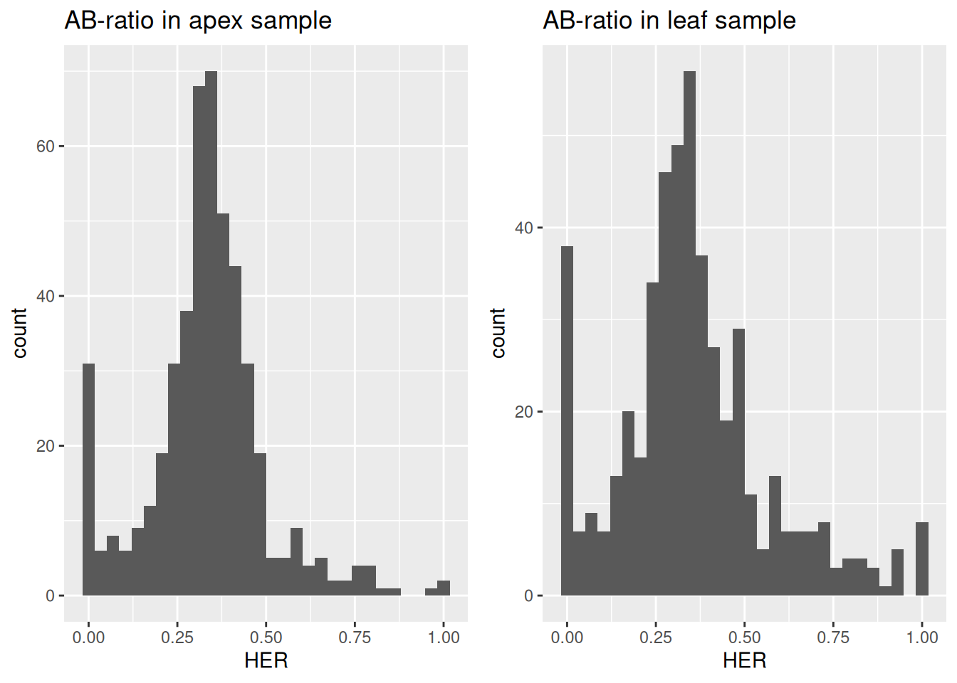
Figure 3.10: Distribution of homeolog expression ratios of D-subgenome between shoot apex and leaf in wheat.
The resulting distributions show a peak around one-thirds, indicating that most homeologs are expressed equally between the D-subgenome and the combined A- and B-subgenomes.
HOBIT can then be applied to the combined dataset as below.
x_ABvsD_output <- hobit(x_ABvsD)
x_ABvsD_output$pvalue[is.na(x_ABvsD_output$pvalue)] <- 1
x_ABvsD_output$qvalue[is.na(x_ABvsD_output$qvalue)] <- 1## gene pvalue qvalue raw_pvalue raw_qvalue D__D__(apex-leaf) D__A+B__(apex-leaf) OR__D__(apex/leaf) OR__A+B__(apex/leaf) Dmax ORmax theta0__D theta0__A+B theta1__D__apex theta1__A+B__apex theta1__D__leaf theta1__A+B__leaf logLik_H0 logLik_H1
## 6 TraesCS1A02G072800 2.526108e-14 9.071842e-12 8.139921e-20 3.463009e-17 -0.4810779 0.4810779 0.1181427 8.46433759 0.4810779 8.464338 0.5489059 0.4510941 0.3060545 0.6939455 0.79108059 0.2089194 -71.44894 -29.99553
## 62 TraesCS1A02G445500 3.772076e-14 9.071842e-12 1.439920e-19 3.463009e-17 -0.2488910 0.2488910 0.3602295 2.77600831 0.2488910 2.776008 0.4712735 0.5287265 0.3465822 0.6534178 0.59541975 0.4045802 -110.88134 -70.13434
## 107 TraesCS2A02G262400 2.774477e-12 3.365049e-10 6.496119e-17 7.907400e-15 -0.5179675 0.5179675 0.1001856 9.98147700 0.5179675 9.981477 0.4979254 0.5020746 0.2369353 0.7630647 0.75605309 0.2439469 -67.24040 -32.59869
## 355 TraesCS5A02G352700 2.798378e-12 3.365049e-10 6.575800e-17 7.907400e-15 0.3532358 -0.3532358 8.0094922 0.12485186 0.3532358 8.009492 0.2719739 0.7280261 0.4498670 0.5501330 0.09245644 0.9075436 -70.04077 -35.01797
## 441 TraesCS7A02G209600 4.948414e-12 4.760374e-10 1.478475e-16 1.422293e-14 0.2540367 -0.2540367 19.1622230 0.05218602 0.2540367 19.162223 0.1474837 0.8525163 0.2742134 0.7257866 0.01932109 0.9806789 -85.42804 -51.45077
## 268 TraesCS4A02G250600 8.431347e-11 6.759130e-09 8.306025e-15 6.658664e-13 -0.2860572 0.2860572 0.3062431 3.26538000 0.2860572 3.265380 0.4729368 0.5270632 0.3300100 0.6699900 0.61553641 0.3844636 -68.41571 -38.28623The detection results can be visualized as follows.
is_sig <- ifelse(x_ABvsD_output$qvalue < 0.01, "q<0.01", "q>=0.01")
plot_HER(x_ABvsD, label = is_sig)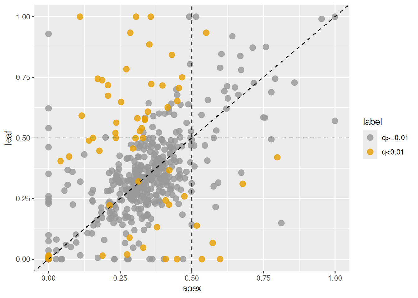
Figure 3.11: Changes in homeolog expression ratios of the D-subgenome versus the combined A- and B-subgenomes between shoot apex and leaf tissues. Each point represents the ratio in shoot apex (x-axis) and leaf (y-axis). Orange points indicate homeologs with significant changes, gray points indicate homeologs without significant changes.
3.2.5 Analysis Environment
## R version 4.5.2 (2025-10-31)
## Platform: x86_64-pc-linux-gnu
## Running under: Ubuntu 24.04.3 LTS
##
## Matrix products: default
## BLAS:   /usr/lib/x86_64-linux-gnu/openblas-pthread/libblas.so.3
## LAPACK: /usr/lib/x86_64-linux-gnu/openblas-pthread/libopenblasp-r0.3.26.so;  LAPACK version 3.12.0
##
## locale:
##  [1] LC_CTYPE=C.UTF-8       LC_NUMERIC=C           LC_TIME=C.UTF-8        LC_COLLATE=C.UTF-8     LC_MONETARY=C.UTF-8
##  [6] LC_MESSAGES=C.UTF-8    LC_PAPER=C.UTF-8       LC_NAME=C              LC_ADDRESS=C           LC_TELEPHONE=C
## [11] LC_MEASUREMENT=C.UTF-8 LC_IDENTIFICATION=C
##
## time zone: UTC
## tzcode source: system (glibc)
##
## attached base packages:
## [1] stats     graphics  grDevices utils     datasets  methods   base
##
## other attached packages:
## [1] UpSetR_1.4.0    plotly_4.11.0   gridExtra_2.3   ggplot2_4.0.1   hespresso_1.0.4
##
## loaded via a namespace (and not attached):
##  [1] gtable_0.3.6         tensorA_0.36.2.1     xfun_0.55            bslib_0.9.0          htmlwidgets_1.6.4
##  [6] processx_3.8.6       lattice_0.22-7       crosstalk_1.2.2      vctrs_0.6.5          tools_4.5.2
## [11] ps_1.9.1             generics_0.1.4       parallel_4.5.2       tibble_3.3.0         cmdstanr_0.9.0
## [16] pkgconfig_2.0.3      data.table_1.18.0    checkmate_2.3.3      RColorBrewer_1.1-3   S7_0.2.1
## [21] distributional_0.5.0 lifecycle_1.0.4      compiler_4.5.2       farver_2.1.2         progress_1.2.3
## [26] statmod_1.5.1        codetools_0.2-20     htmltools_0.5.9      sass_0.4.10          lazyeval_0.2.2
## [31] yaml_2.3.12          tidyr_1.3.2          pillar_1.11.1        crayon_1.5.3         jquerylib_0.1.4
## [36] cachem_1.1.0         limma_3.66.0         abind_1.4-8          parallelly_1.46.0    posterior_1.6.1.9000
## [41] tidyselect_1.2.1     locfit_1.5-9.12      digest_0.6.39        future_1.68.0        purrr_1.2.0
## [46] dplyr_1.1.4          bookdown_0.46        listenv_0.10.0       labeling_0.4.3       splines_4.5.2
## [51] fastmap_1.2.0        grid_4.5.2           cli_3.6.5            magrittr_2.0.4       future.apply_1.20.1
## [56] edgeR_4.8.1          withr_3.0.2          prettyunits_1.2.0    scales_1.4.0         backports_1.5.0
## [61] httr_1.4.7           rmarkdown_2.30       globals_0.18.0       otel_0.2.0           progressr_0.18.0
## [66] hms_1.1.4            evaluate_1.0.5       knitr_1.51           viridisLite_0.4.2    rlang_1.1.6
## [71] Rcpp_1.1.0           glue_1.8.0           rstudioapi_0.17.1    jsonlite_2.0.0       plyr_1.8.9
## [76] R6_2.6.1