5.2 Simulating Allohexaploid Data

To simulate read counts for an allohexaploid with three subgenomes, set n_subgenomes = 3. In this case, the mean and dispersion parameters are derived from real RNA-Seq data of allohexaploid wheat (Yang et al. 2021).

x <- sim_homeolog_counts(n_subgenomes = 3)

Simulation parameters can be retrieved using the get_sim_params() function, and ground-truth homeologs with significant expression ratio shifts can be defined using the def_sigShift(), similar to the allotetraploid example.

For exmaple, using the def_sigShift() function can define ground-truth RSHs, homeologs with large changes satisfied the given thresholds in any subgenome.

is_sig <- def_sigShift(x, Dmax = 0.2, ORmax = 2, operator = "OR")
table(is_sig)

## is_sig
## FALSE  TRUE 
##  9091   909

To define shifts specific to a single subgenome (e.g., the first subgenome), set the base argument accordingly as follows.

x <- sim_homeolog_counts(n_subgenomes = 3)

is_sig <- def_sigShift(x, base = 1, Dmax = 0.2, ORmax = 2, operator = "OR")
table(is_sig)

## is_sig
## FALSE  TRUE 
##  9577   423

Visualization of allohexaploid data, comprising three subgenomes, follows a similar workflow as for allotetraploids. To display the distribution of expression ratios for the first subgenome, run as follows.

x <- sim_homeolog_counts(n_subgenomes = 3)
distr_plots_1 <- plot_HER_distr(x)
names(distr_plots_1)

## [1] "group_1" "group_2"

library(ggplot2)
library(gridExtra)
grid.arrange(distr_plots_1[["group_1"]] + ggtitle("group_1 on 1st subgenome"), 
             distr_plots_1[["group_2"]] + ggtitle("group_2 on 1st subgenome"),
             ncol = 2)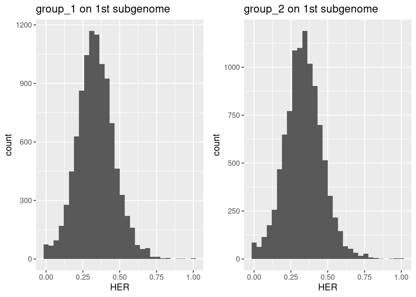

Figure 5.4: Distribution of homeolog expression ratios for the first subgenome in a simulated allohexaploid across two groups.

Users can specify which subgenome to use for calculating expression ratios with the base argument. For example, to visualize ratios for the second or third subgenome, run as follows.

distr_plots_2 <- plot_HER_distr(x, base = 2)
distr_plots_3 <- plot_HER_distr(x, base = 3)

grid.arrange(distr_plots_1[["group_1"]] + ggtitle("group_1 on #1"),
             distr_plots_1[["group_2"]] + ggtitle("group_2 on #1"),
             distr_plots_2[["group_1"]] + ggtitle("group_1 on #2"),
             distr_plots_2[["group_2"]] + ggtitle("group_2 on #2"),
             distr_plots_3[["group_1"]] + ggtitle("group_1 on #3"),
             distr_plots_3[["group_2"]] + ggtitle("group_2 on #3"),
             ncol = 2)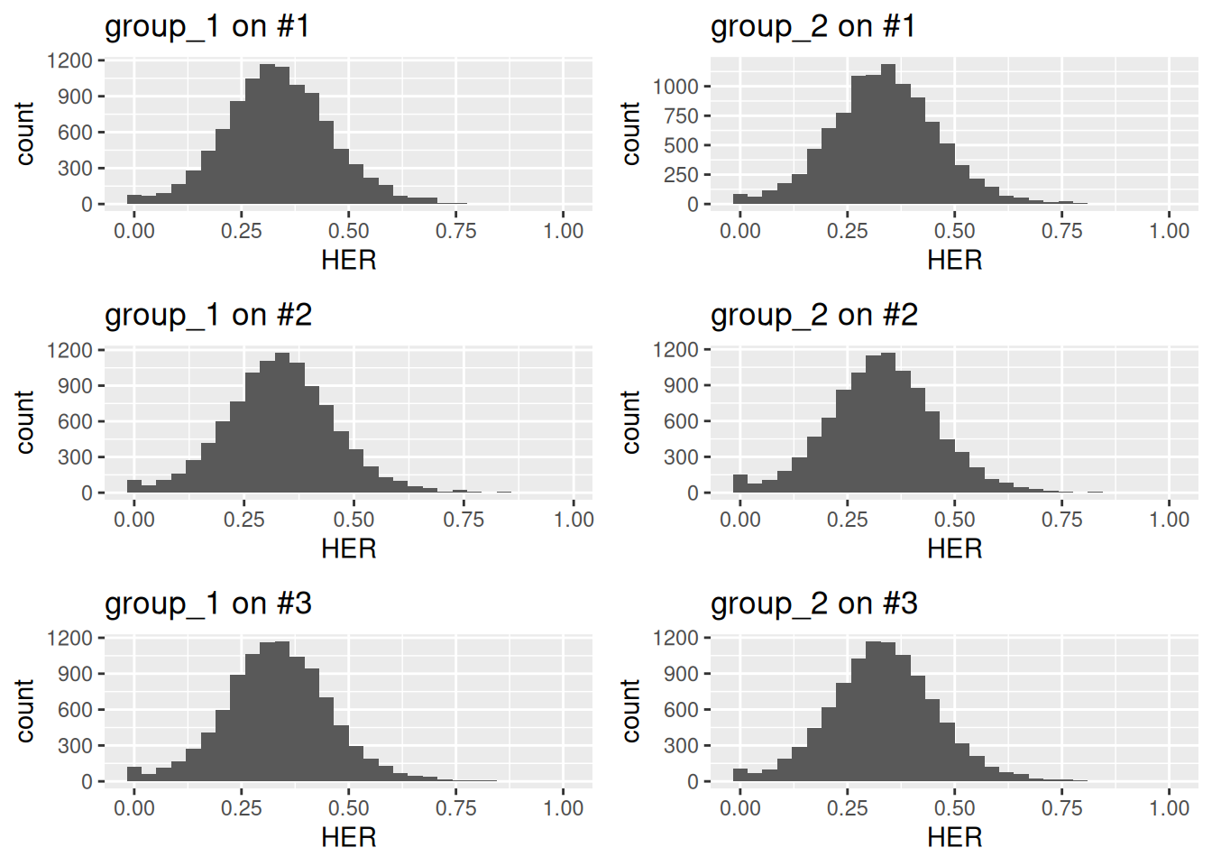

Figure 5.5: Distribution of homeolog expression ratios for all subgenomes in a simulated allohexaploid across two groups.

The plot_HER() function also works for allohexaploids. By default, it plots expression ratios for the first subgenome.

plot_HER(x, alpha = 0.3)

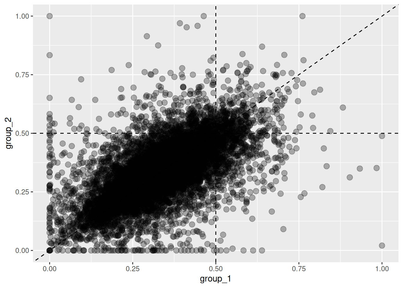
Figure 5.6: Changes in homeolog expression ratios of the first subgenome between two groups. Each point represents the expression ratio of the first subgenome in both groups.

To plot ratios for a specific subgenome, set the base argument. For example, to visualize the second subgenome, run as follows.

plot_HER(x, base = 2, alpha = 0.3)

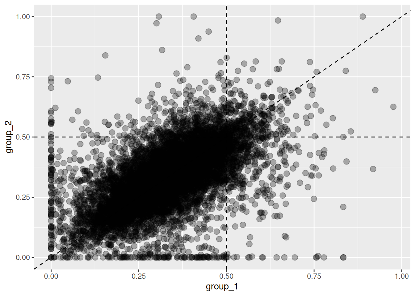
Figure 5.7: Changes in homeolog expression ratios of the second subgenome between two groups. Each point represents the expression ratio of the second subgenome in both groups.

Ground-truth shifts can be highlighted in the scatter plot using def_sigShift(). By default, shifts are defined across all subgenomes, so some homeologs may appear highlighted even if changes in the plotted subgenome are minor.

is_sig <- def_sigShift(x, base = 0, Dmax = 0.2, ORmax = 2)
plot_HER(x, label = is_sig, alpha = 0.3)

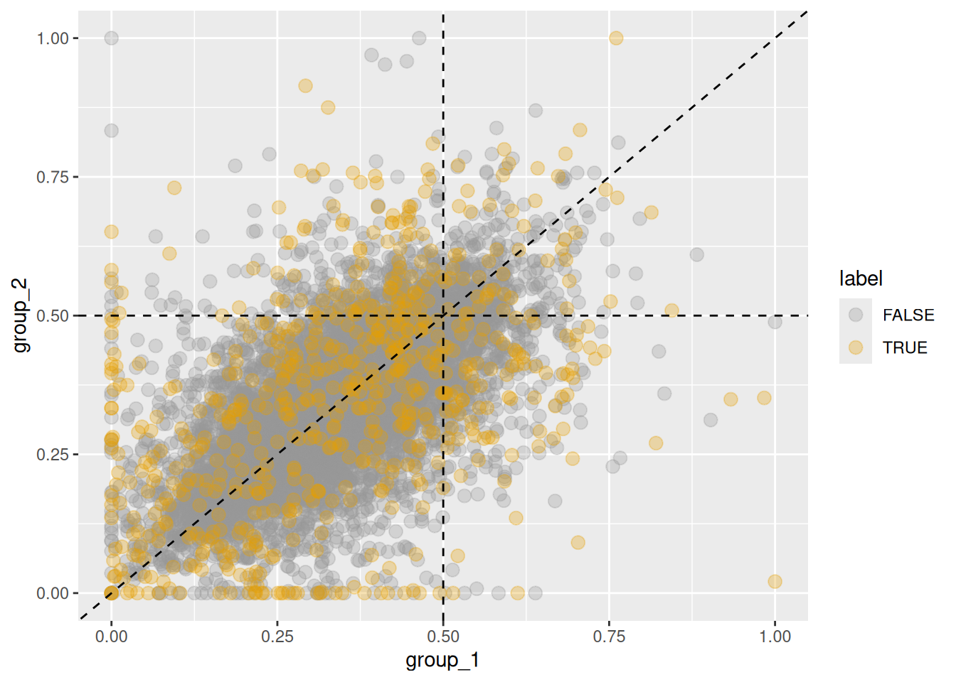
Figure 5.8: Changes in homeolog expression ratios of the first subgenome between two groups. Orange points indicate homeologs with significant changes in any subgenome, while gray points indicate no significant change.

To highlight only homeologs that meet the thresholds in a specific subgenome, specify the base argument.

is_sig_b1 <- def_sigShift(x, base = 1, Dmax = 0.2, ORmax = 1.8)
plot_HER(x, base = 1, label = is_sig_b1, alpha = 0.3)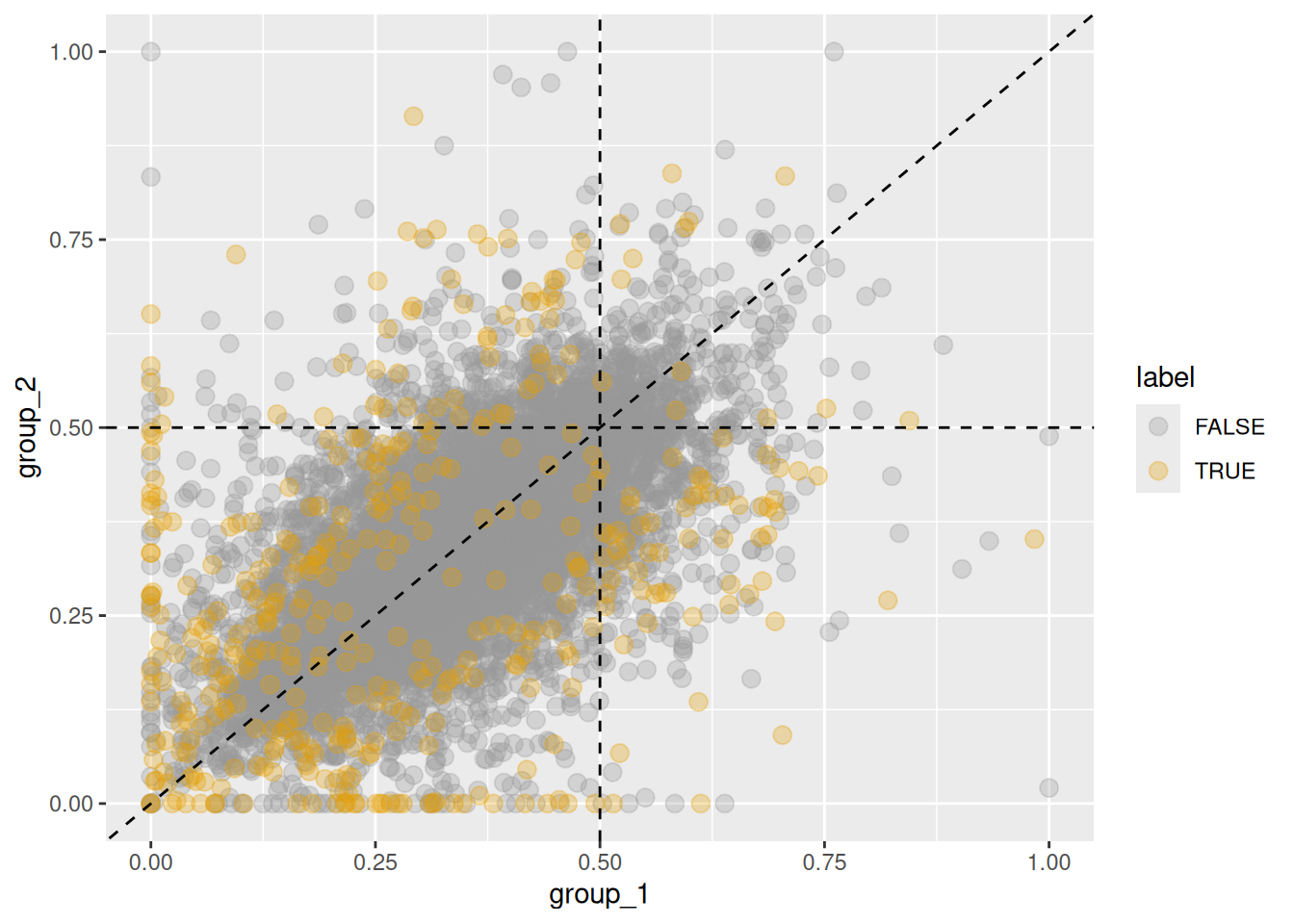

Figure 5.9: Changes in homeolog expression ratios of the first subgenome between two groups. Orange points indicate homeologs with significant changes in the first subgenome, while gray points show no significant change.