3.1 Allohexaploid C. flexuosa
3.1.1 Introduction
Cardamine flexuosa (2n = 4x = 32, HHAA), wavy bittercress, is an allopolyploid species that originated from two diploid progenitors, Cardamine hirsuta (2n = 2x = 16, HH) and Cardamine amara (2n = 2x = 16, AA) (Mandáková et al. 2014). While C. hirsuta is typically adapted to dry habitats such as roadsides, C. amara inhabits wet environments such as riversides or running streams. The allopolyploid C. flexuosa thrives across a wide range of ecological habitats.
Akiyama et al. conducted an RNA-seq experiment using leaf samples of C. flexuosa collected from wet and dry habitats across three different days (Akiyama et al. 2021). Each habitat–date combination included two or three biological replicates. In the original study, homeolog expression levels were quantified using read counts processed through the HomeoRoq sorting pipeline (Akama et al. 2014). Analysis of homeolog expression ratios revealed that a small percentage of homeologs in C. flexuosa exhibit shifts in expression depending on environmental differences, wet and dry.
3.1.2 Data Preparation
In this example, we demonstrate how to use HOBIT and HomeoRoq
to analyze this C. flexuosa dataset.
To reduce computation time, we focus on samples collected on May 16, 2013,
and randomly select 500 homeolog pairs (c_flexuosa.0516.mini.txt.gz).
Users can, however, analyze the full dataset or samples from other dates,
which are available in the data directory,
and the same workflow can be applied.
gexp <- read.table("../data/c_flexuosa.0516.mini.txt.gz",
                   header = TRUE, sep = "\t", row.names = 1)
head(gexp)
## wet_1 wet_2 wet_3 dry_1 dry_2 dry_3
## CARHR000190_H 126 109 150 175 113 124
## CARHR000660_H 3 4 8 10 2 5
## CARHR000770_H 129 95 170 233 316 238
## CARHR000890_H 45 32 117 5 6 1
## CARHR001940_H 23 22 73 176 46 108
## CARHR003740_H 541 436 576 552 344 284Next, load the homeolog mapping table, which links gene expression to their corresponding homeologs. This table is a tab-separated file in which the first and second columns represent gene names from C. hirsuta and C. amara, respectively.
mapping_table <- read.table("../data/c_flexuosa.homeolog.txt.gz",
                            header = TRUE, sep = "\t")
head(mapping_table)
## C_hirsuta C_amara
## 1 CARHR000010_H CARHR000010_A
## 2 CARHR000060_H CARHR000060_A
## 3 CARHR000070_H CARHR000070_A
## 4 CARHR000090_H CARHR000090_A
## 5 CARHR000110_H CARHR000110_A
## 6 CARHR000120_H CARHR000120_AWe then use the newExpMX() function
to organize the gene expression matrix (gexp) into a homeolog expression matrix
using the mapping table (mapping_table) and store the result in an ExpMX class object.
## # 2 subgenome sets (C_hirsuta, C_amara)
## # 500 homeolog tuples
## ---------------------
## Experiment Design:
##   group
## 1   wet
## 2   wet
## 3   wet
## 4   dry
## 5   dry
## 6   dry
## ---------------------
## > subgenome: C_hirsuta
##      [,1] [,2] [,3] [,4] [,5] [,6]
## [1,]  126  109  150  175  113  124
## [2,]    3    4    8   10    2    5
## [3,]  129   95  170  233  316  238
## [4,]   45   32  117    5    6    1
## [5,]   23   22   73  176   46  108
## [6,]  541  436  576  552  344  284
## +++++++++++++++++++++
## > subgenome: C_amara
##      [,1] [,2] [,3] [,4] [,5] [,6]
## [1,]  238  141   82  136   63   88
## [2,]   14   10   24   23    6   13
## [3,]   20    9   17   26   40   22
## [4,]   23   19   73    2    5    2
## [5,]   15   17   54  209   36   70
## [6,]  798  610  880  958  969  567
## ---------------------
Before performing the test,
we normalize the raw read counts using the TMM method (Robinson and Oshlack 2010)
to adjust for differences in library size.
However, if the expression data (gexp) has already been normalized (e.g. FPKM),
this step can be skipped.
To visualize the distributions of homeolog expression ratios,
use the plot_HER_distr() function.
This function returns a list of histograms, one for each condition,
showing the distribution of homeolog expression ratios.
## [1] "wet" "dry"By default, the expression ratio is calculated as the proportion contributed
by the first subgenome relative to all subgenomes.
In this dataset, the first subgenome is derived from C. hirsuta,
as indicated by the first column in the mapping table (mapping_table).
To display the distribution of homeolog expression ratios for each experimental group, run the following code.
library(ggplot2)
library(gridExtra)
grid.arrange(distr_plots[["wet"]] + ggtitle("wet"),
             distr_plots[["dry"]] + ggtitle("dry"),
             ncol = 2)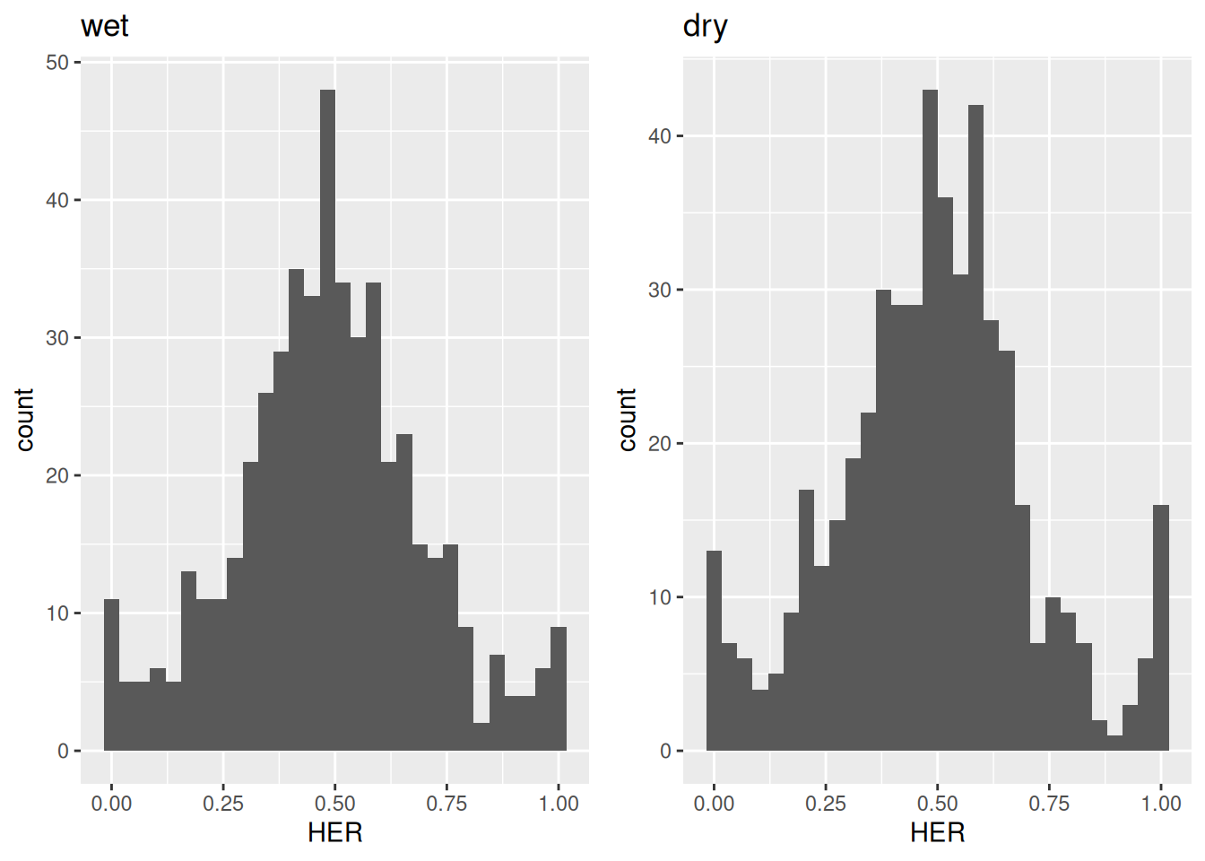
Figure 3.1: Distribution of homeolog expression ratios in C. flexuosa under wet and dry habitats.
After visually inspecting the distributions, if no irregularities are observed, users can proceed to apply the statistical test.
3.1.3 HOBIT
HOBIT can be executed using the hobit() function, which performs a statistical test
to detect homeologs with shifts in expression ratios between wet and dry habitats.
This step takes approximately five minutes
using eight threads and may vary depending on hardware performance.
The order of the test output matches that of the input.
##            gene    pvalue qvalue raw_pvalue raw_qvalue D__C_hirsuta__(dry-wet) D__C_amara__(dry-wet) OR__C_hirsuta__(dry/wet) OR__C_amara__(dry/wet)       Dmax    ORmax theta0__C_hirsuta theta0__C_amara theta1__C_hirsuta__dry theta1__C_amara__dry theta1__C_hirsuta__wet theta1__C_amara__wet logLik_H0 logLik_H1
## 1 CARHR000190_H 0.1257453      1  0.0671578  0.7994976              0.13851574           -0.13851574                1.7524086              0.5706432 0.13851574 1.752409         0.5145677       0.4854323              0.5851042            0.4148958              0.4456696            0.5543304 -64.62743 -63.01814
## 2 CARHR000660_H 1.0000000      1  1.0000000  1.0000000              0.05785510           -0.05785509                1.3678354              0.7310821 0.05785510 1.367835         0.2535746       0.7464254              0.2815327            0.7184673              0.2193108            0.7806892 -31.63977 -31.90169
## 3 CARHR000770_H 1.0000000      1  1.0000000  1.0000000              0.00042667           -0.00042667                1.0041632              0.9958542 0.00042667 1.004163         0.8931450       0.1068550              0.8953420            0.1046580              0.8948587            0.1051413 -53.31894 -53.65784
## 4 CARHR000890_H 0.7523488      1  0.7059717  1.0000000             -0.07999806            0.07999806                0.7076250              1.4131778 0.07999806 1.413178         0.5882221       0.4117779              0.5494622            0.4505378              0.6321275            0.3678725 -41.38102 -41.42952
## 5 CARHR001940_H 1.0000000      1  1.0000000  1.0000000             -0.04958549            0.04958549                0.8155551              1.2261587 0.04958549 1.226159         0.5514201       0.4485799              0.5273460            0.4726540              0.5761417            0.4238583 -57.12549 -57.46951
## 6 CARHR003740_H 0.3571554      1  0.2709275  1.0000000             -0.08852804            0.08852804                0.6771142              1.4768559 0.08852804 1.476856         0.3603599       0.6396401              0.3148542            0.6851458              0.4043972            0.5956028 -75.30201 -74.68230
Note that the pvalue and qvalue columns in x_output may contain NA values.
This happens when at least one gene in a homeolog pair is not expressed in one or more conditions,
making it impossible to calculate expression ratios.
As a result, the statistical test cannot be performed for those pairs.
These NA values may affect sorting or counting the number of significant homeolog pairs.
Therefore, we recommend replacing NA with 1 (i.e., non-significant)
before performing downstream analyses.
To rank the output in descending order of p-values, use the following code.
##              gene       pvalue       qvalue   raw_pvalue   raw_qvalue D__C_hirsuta__(dry-wet) D__C_amara__(dry-wet) OR__C_hirsuta__(dry/wet) OR__C_amara__(dry/wet)      Dmax      ORmax theta0__C_hirsuta theta0__C_amara theta1__C_hirsuta__dry theta1__C_amara__dry theta1__C_hirsuta__wet theta1__C_amara__wet  logLik_H0  logLik_H1
## 318 CARHR189440_H 1.129813e-14 5.649065e-12 2.591104e-20 1.295552e-17              -0.2451507             0.2451507              0.006851859            145.9457876 0.2451507 145.945788         0.8741883       0.1258117              0.7517053            0.2482947             0.99759706          0.002402937 -138.38913  -95.78485
## 299 CARHR177020_H 5.916810e-07 1.479203e-04 2.360346e-09 5.900866e-07              -0.4688876             0.4688876              0.066520772             15.0328988 0.4688876  15.032899         0.6883111       0.3116889              0.4546812            0.5453188             0.92461027          0.075389728  -64.98708  -47.22464
## 460 CARHR262780_H 6.476010e-06 8.827291e-04 6.947355e-08 9.813714e-06              -0.5230227             0.5230227              0.083224955             12.0156290 0.5230227  12.015629         0.4200055       0.5799945              0.1529102            0.8470898             0.68445069          0.315549310  -91.09666  -76.77417
## 118 CARHR064090_H 7.061832e-06 8.827291e-04 7.850971e-08 9.813714e-06              -0.3483715             0.3483715              0.169307356              5.9064180 0.3483715   5.906418         0.3199125       0.6800875              0.1415246            0.8584754             0.49480641          0.505193585 -115.63690 -101.50720
## 442 CARHR252830_H 2.240475e-05 2.240475e-03 4.003070e-07 4.003070e-05               0.4969540            -0.4969540             49.176778705              0.0203348 0.4969540  49.176788         0.7162030       0.2837970              0.9777606            0.0222394             0.46669610          0.533303900  -55.68348  -43.13537
## 52  CARHR027460_H 7.048256e-05 5.873546e-03 2.012282e-06 1.676902e-04               0.1569487            -0.1569487              5.501958555              0.1817535 0.1569487   5.501959         0.1238240       0.8761760              0.2017059            0.7982941             0.04398341          0.956016585  -69.21729  -58.12450
To visualize homeologs with shifts in expression ratios between wet and dry habitats,
use the plot_HER() function.
This function generates a scatter plot comparing the expression ratios
calculated for the wet and dry groups.
By default, the expression ratio is defined as the proportion contributed
by the first subgenome (i.e., the subgenome derived from C. hirsuta)
relative to the total expression across all subgenomes.
In the example below, homeologs with q-values less than 0.01 are highlighted.
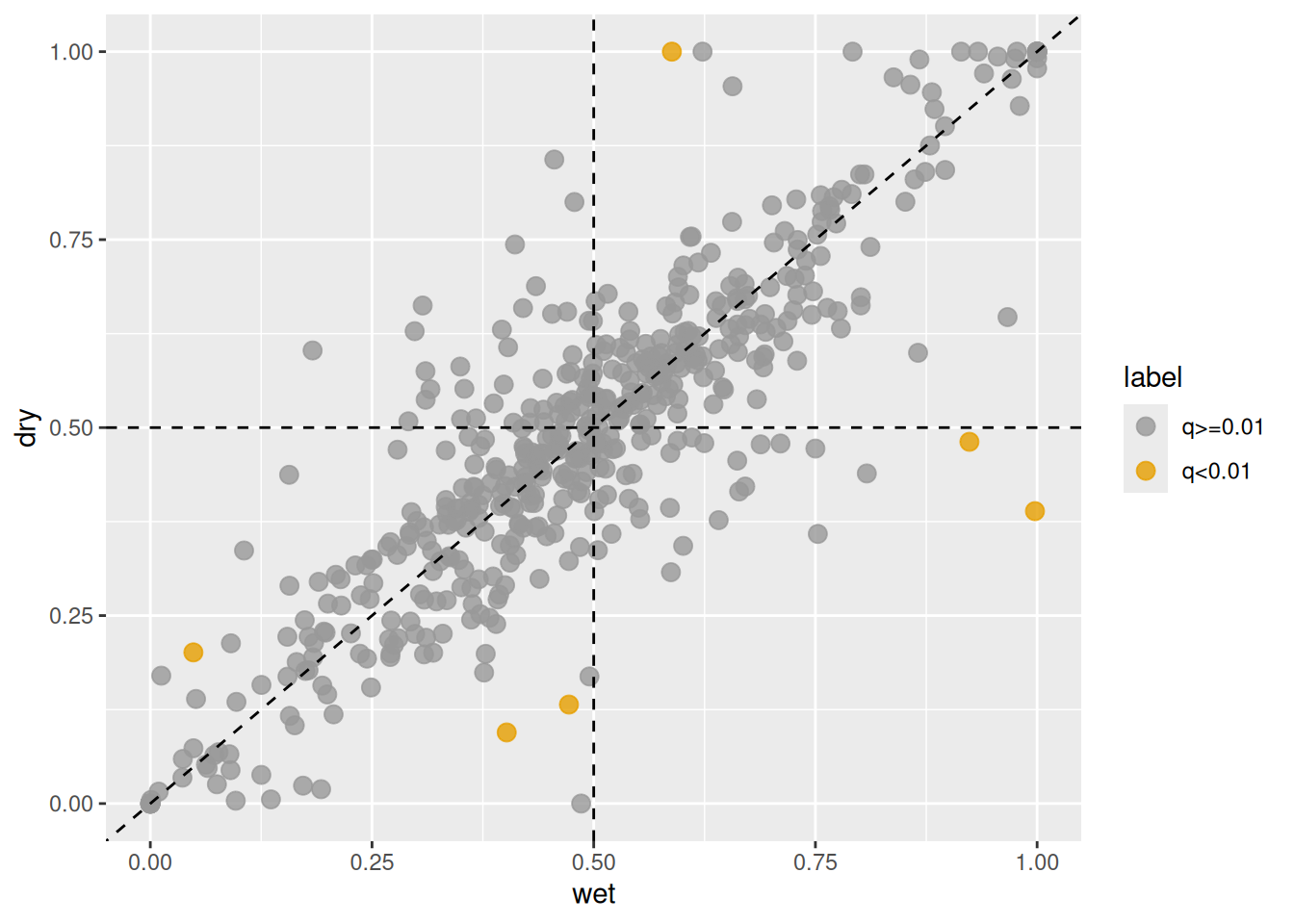
Figure 3.2: Changes in homeolog expression ratios between wet (x-axis) and dry (y-axis) habitats. Orange points indicate homeologs with significant shifts detected by HOBIT, while gray points represent homeologs without significant changes.
The plot generated by the plot_HER() function can also be visualized using plotly,
enabling interactive exploration of individual homeologs.
The interactive interface allows users to zoom in on specific regions of interest,
and hovering over data points displays detailed information for each homeolog.
Figure 3.3: Visualization of homeolog expression ratio shifts with plotly.
3.1.4 HomeoRoq
For allopolyploids composed of two subgenomes under two different conditions,
HomeoRoq is also a suitable option for detecting homeologs with shifts in expression ratios.
It can be executed using the homeoroq() function in the same way as hobit(),
as shown below.
x_homeoroq <- homeoroq(x)
x_homeoroq$pvalue[is.na(x_homeoroq$pvalue)] <- 1
x_homeoroq$qvalue[is.na(x_homeoroq$qvalue)] <- 1## gene pvalue qvalue sumexp__wet__C_hirsuta sumexp__wet__C_amara sumexp__dry__C_hirsuta sumexp__dry__C_amara ratio__wet__C_hirsuta ratio__dry__C_hirsuta ratio_sd
## 52 CARHR027460_H 0 0 41.57096 909.51163 102.245685 409.2047 0.0437091 0.10105752 0.07791076
## 68 CARHR034170_H 0 0 55.84898 207.90394 4.376849 213.3613 0.2117473 0.02061821 0.13132195
## 118 CARHR064090_H 0 0 2317.24730 2368.74631 658.880578 4368.6664 0.4945050 0.21762278 0.21895848
## 211 CARHR120540_H 0 0 58.59614 35.50623 21.889335 0.0000 0.6226851 0.38137679 0.18669063
## 299 CARHR177020_H 0 0 173.87466 14.80519 152.537840 173.6894 0.9215327 0.91152790 0.22859512
## 307 CARHR184910_H 0 0 60.88312 274.91276 5.699047 801.7122 0.1813099 0.02030936 0.12764240The overlap of homeologs with shifts in expression ratios detected by HOBIT and HomeoRoq can be visualized using an UpSet plot, which is implemented in the UpSetR package (Conway et al. 2017).
library(UpSetR)
sig_homeologs <- list(
    HOBIT = x_output$gene[x_output$qvalue < 0.01],
    HomeoRoq = x_homeoroq$gene[x_homeoroq$qvalue < 0.01]
)
upset(fromList(sig_homeologs))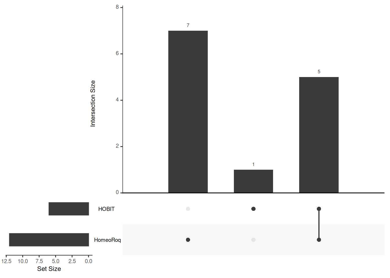
Figure 3.4: Overlap of homeologs with shifted expression ratios detected by HOBIT and HomeoRoq.
Additionally, homeologs with shifts in expression ratios detected by both methods
can be visualized using the plot_HER() function.
is_sig <- rep("n.s.", length = nrow(x_output))
is_sig[x_output$qvalue < 0.01] <- "HOBIT"
is_sig[x_homeoroq$qvalue < 0.01] <- "HomeoRoq"
is_sig[x_output$qvalue < 0.01 & x_homeoroq$qvalue < 0.01] <- "HOBIT&HomeoRoq"
is_sig <- factor(is_sig, levels = c("n.s.", "HOBIT", "HomeoRoq", "HOBIT&HomeoRoq"))
plot_HER(x, label = is_sig)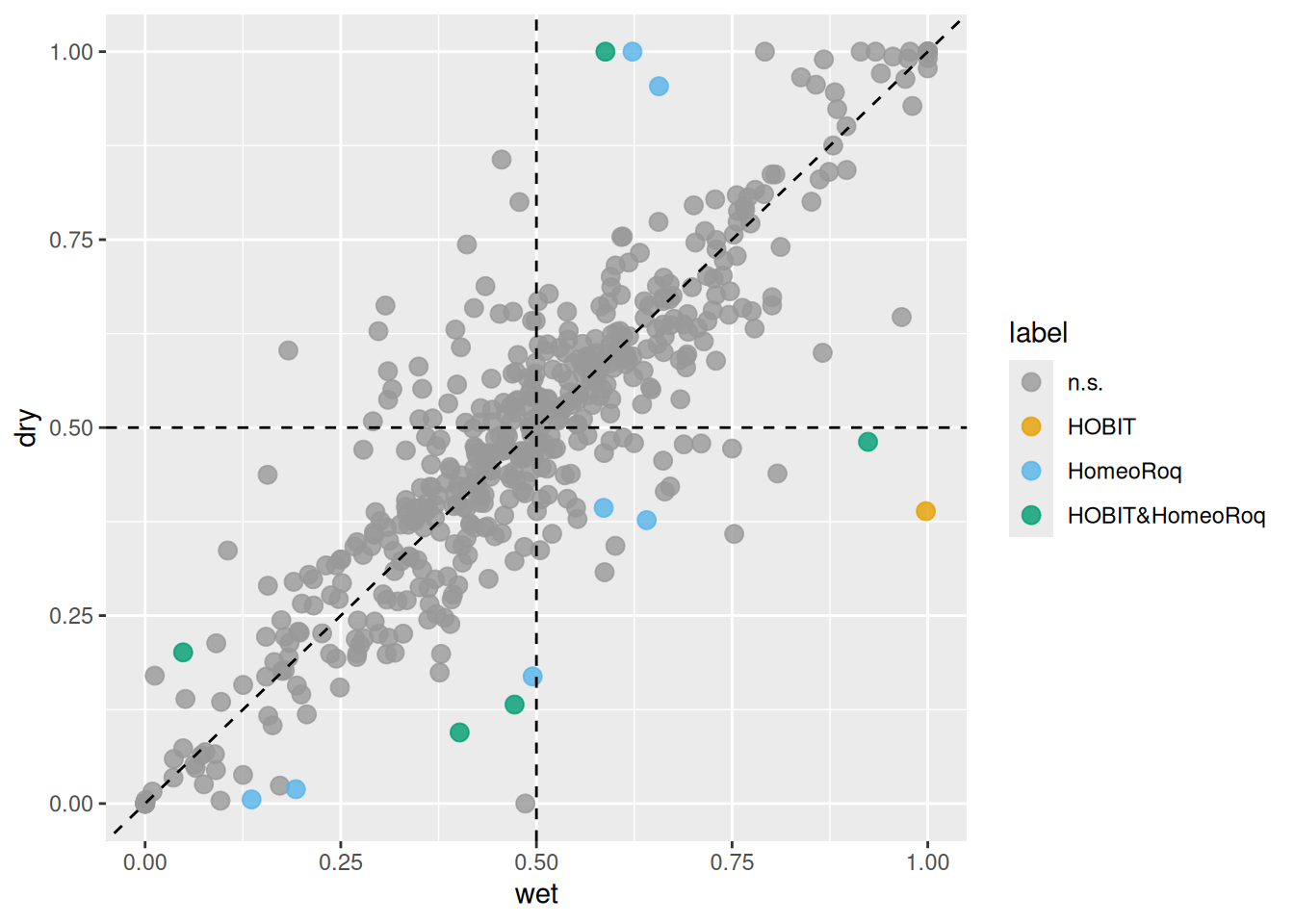
Figure 3.5: Comparison of homeologs with changes in expression ratios detected by HOBIT and HomeoRoq. Each point represents a homeolog expression ratio in wet (x-axis) and dry (y-axis) conditions. Points labeled as n.s. indicate homeologs without significant changes detected by either method; other points represent homeologs identified as having significant changes by the respective method.
3.1.5 Analysis Environment
## R version 4.5.2 (2025-10-31)
## Platform: x86_64-pc-linux-gnu
## Running under: Ubuntu 24.04.3 LTS
##
## Matrix products: default
## BLAS:   /usr/lib/x86_64-linux-gnu/openblas-pthread/libblas.so.3
## LAPACK: /usr/lib/x86_64-linux-gnu/openblas-pthread/libopenblasp-r0.3.26.so;  LAPACK version 3.12.0
##
## locale:
##  [1] LC_CTYPE=C.UTF-8       LC_NUMERIC=C           LC_TIME=C.UTF-8        LC_COLLATE=C.UTF-8     LC_MONETARY=C.UTF-8
##  [6] LC_MESSAGES=C.UTF-8    LC_PAPER=C.UTF-8       LC_NAME=C              LC_ADDRESS=C           LC_TELEPHONE=C
## [11] LC_MEASUREMENT=C.UTF-8 LC_IDENTIFICATION=C
##
## time zone: UTC
## tzcode source: system (glibc)
##
## attached base packages:
## [1] stats     graphics  grDevices utils     datasets  methods   base
##
## other attached packages:
## [1] UpSetR_1.4.0    plotly_4.11.0   gridExtra_2.3   ggplot2_4.0.1   hespresso_1.0.4
##
## loaded via a namespace (and not attached):
##  [1] gtable_0.3.6         tensorA_0.36.2.1     xfun_0.55            bslib_0.9.0          htmlwidgets_1.6.4
##  [6] processx_3.8.6       lattice_0.22-7       crosstalk_1.2.2      vctrs_0.6.5          tools_4.5.2
## [11] ps_1.9.1             generics_0.1.4       parallel_4.5.2       tibble_3.3.0         cmdstanr_0.9.0
## [16] pkgconfig_2.0.3      data.table_1.18.0    checkmate_2.3.3      RColorBrewer_1.1-3   S7_0.2.1
## [21] distributional_0.5.0 lifecycle_1.0.4      compiler_4.5.2       farver_2.1.2         progress_1.2.3
## [26] statmod_1.5.1        codetools_0.2-20     htmltools_0.5.9      sass_0.4.10          lazyeval_0.2.2
## [31] yaml_2.3.12          tidyr_1.3.2          pillar_1.11.1        crayon_1.5.3         jquerylib_0.1.4
## [36] cachem_1.1.0         limma_3.66.0         abind_1.4-8          parallelly_1.46.0    posterior_1.6.1.9000
## [41] tidyselect_1.2.1     locfit_1.5-9.12      digest_0.6.39        future_1.68.0        purrr_1.2.0
## [46] dplyr_1.1.4          bookdown_0.46        listenv_0.10.0       labeling_0.4.3       splines_4.5.2
## [51] fastmap_1.2.0        grid_4.5.2           cli_3.6.5            magrittr_2.0.4       future.apply_1.20.1
## [56] edgeR_4.8.1          withr_3.0.2          prettyunits_1.2.0    scales_1.4.0         backports_1.5.0
## [61] httr_1.4.7           rmarkdown_2.30       globals_0.18.0       otel_0.2.0           progressr_0.18.0
## [66] hms_1.1.4            evaluate_1.0.5       knitr_1.51           viridisLite_0.4.2    rlang_1.1.6
## [71] Rcpp_1.1.0           glue_1.8.0           rstudioapi_0.17.1    jsonlite_2.0.0       plyr_1.8.9
## [76] R6_2.6.1